
刚体旋转:环流
几何画板及绘图内容加载中,请稍等……
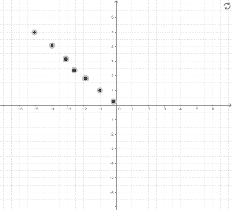
①本范例演示刚体旋转的流场图形现象;②涉及核心数学概念包括向量场、速度分布、积分计算;③构造要点:运用了Textfield, SolveODE, Sequence, SlopeField, Midpoint, SelectedIndex, Element, CurveCartesian, Sum, Segment, Line等GeoGebra命令与对象;④适合高中及以上学生及数学爱好者学习刚体运动与流体力学。
GeoGebra 命令及参数
Textfield(x_{min}) → inputBox2Textfield(x_{max}) → inputBox3Textfield(y_{min}) → inputBox4Textfield(y_{max}) → inputBox5SolveODE(f, x(A), y(A), x_{max}, 0.01) → SLVFSolveODE(f, x(A), y(A), x_{min}, 0.01) → SLVBSequence(SolveODE[f, 0, t1, x_{max}, 0.01], t1, -2, 2, 0.25) → SLVFLSequence(SolveODE[f, 0, t1, x_{min}, 0.01], t1, -2, 2, 0.25) → SLVBLSlopeField(f, n, a, x_{min}, y_{min}, x_{max}, y_{max}) → SFSequence(Sequence[Vector[(j, k), (j + (a * v_x(j, k)), k + (a * v_y(j, k)))], j, x_{min}, x_{max}, xstep], k, y_{min}, y_{max}, ystep) → vFieldSolveODE(f, x(B), y(B), x_{max}, 0.01) → numericalIntegral1SolveODE(f, x(C), y(C), x_{max}, 0.01) → numericalIntegral2SolveODE(f, x(D), y(D), x_{max}, 0.01) → numericalIntegral3Midpoint(K, L) → MSelectedIndex(pathNames) → pathIndexElement(pathList, pathIndex) → pathCurveCartesian(x(path(t)), y(path(t)), t, 0, s) → partPathSequence(Vector[path(s), path(s) + ((a * v_x(x(path(s)), y(path(s)))), (a * v_y(x(path(s)), y(path(s)))))], s, 0, 1, 0.1) → pathVectorsSum(Sequence[((path(i + dS) - path(i)) * (v_x(x(path(i + dS / 2)), y(path(i + dS / 2))), v_y(x(path(i + dS / 2)), y(path(i + dS / 2))))), i, 0, s - dS, dS]) → lineIntegralSegment(path(0.2), path(0.21)) → arrow1Segment(path(0.5), path(0.51)) → arrow2Segment(path(0.8), path(0.81)) → arrow3Textfield(time) → InputBox2SolveODE(f, x(F), y(F), x_{max}, 0.01) → numericalIntegral4SolveODE((-y), x, x(E), y(E), x_{max}, 0.01) → numericalIntegral5CurveCartesian((x(E) * cos((w * t))) - (y(E) * sin((w * t))), (x(E) * sin((w * t))) + (y(E) * cos((w * t))), t, 0, time) → stream_1CurveCartesian((x(A) * cos((w * t))) - (y(A) * sin((w * t))), (x(A) * sin((w * t))) + (y(A) * cos((w * t))), t, 0, time) → stream_2CurveCartesian((x(B) * cos((w * t))) - (y(B) * sin((w * t))), (x(B) * sin((w * t))) + (y(B) * cos((w * t))), t, 0, time) → stream_3CurveCartesian((x(C) * cos((w * t))) - (y(C) * sin((w * t))), (x(C) * sin((w * t))) + (y(C) * cos((w * t))), t, 0, time) → stream_4CurveCartesian((x(D) * cos((w * t))) - (y(D) * sin((w * t))), (x(D) * sin((w * t))) + (y(D) * cos((w * t))), t, 0, time) → stream_5CurveCartesian((x(F) * cos((w * t))) - (y(F) * sin((w * t))), (x(F) * sin((w * t))) + (y(F) * cos((w * t))), t, 0, time) → stream_6CurveCartesian((x(Q) * cos((w * t))) - (y(Q) * sin((w * t))), (x(Q) * sin((w * t))) + (y(Q) * cos((w * t))), t, 0, time) → stream_7Line(S, xAxis) → cLine(T, xAxis) → d
AI 绘图提示语参考
绘制刚体旋转的流场图,展示速度分布和积分计算。首先画出速度场的方向线,用箭头表示在不同点的速度方向和大小。接着,绘制两条对称的曲线,分别代表从最小和最大x值出发的速度轨迹。再添加几条曲线,展示不同初始点的速度轨迹。最后,用流线表示随时间变化的运动轨迹,并标注速度场和轨迹的关键区域。
以上提示语为根据原始绘图命令整理而来,仅供参考。