
线性函数的倒数
几何画板及绘图内容加载中,请稍等……
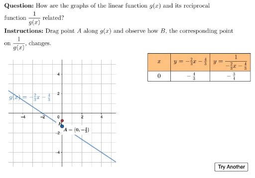
①本范例演示了如何绘制并分析线性函数的倒数图像及其渐近线;②涉及的核心数学概念包括线性函数、倒数函数、渐近线、解析几何;③作图要点提炼自构造摘要,使用了Polygon、Union、LineToSlopeFormRHS、RemoveUndefined、UnicodeToLetter、LaTeX、Point、Line、Zip、TableText等GeoGebra命令和对象;④适合高中阶段学习函数变换和解析几何的学生使用。
GeoGebra 命令及参数
Polygon({(left, top), (right, top), (right, bottom), (left, bottom)}) → viewboxUnion(Sequence[i, i, -5, 5], Zip[xIntercept + A, A, fractions]) → allXvaluesLineToSlopeFormRHS(f) → lineTxtRemoveUndefined(Zip[If[A ≥ minX ∧ A ≤ maxX, A], A, allXvalues]) → useableXvaluesUnicodeToLetter(10007) → xmarkUnicodeToLetter(10003) → cmarkLaTeX("\text{The asymptotes of \(y=\dfrac{1}{g(x)}\) \\occur at the zeros of \(g(x)\). \\The invariant points occur\\when \(y=\pm 1\).}") → fbExplanationLaTeX((((("\text{\textbf{Question: }" * MainInstruc) * "\\\textbf{Instructions: }") * SpecInstruc) * "}")) → allInstrucPoint(Zip[(C, f(C)), C, useableXvalues]) → ALine((xIntercept, 0), yAxis) → vAsymptoteZip((A, f(A)), A, useableXvalues) → useablePointsLaTeX("B") → lblBTableText({titles, dataRow}, "|_c") → dataTable