
勾股定理的重组证明
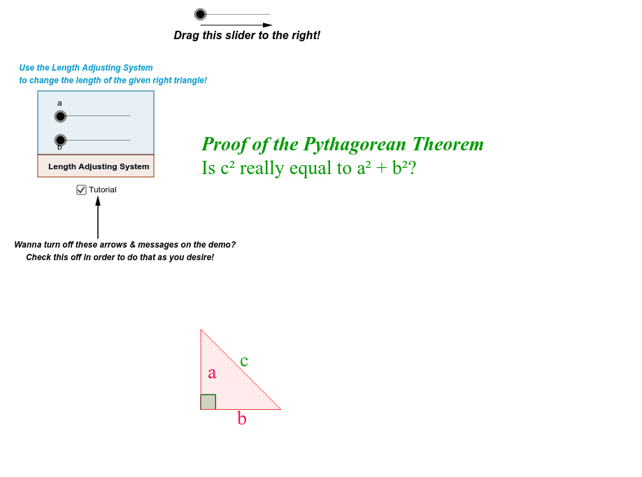
几何画板及绘图内容加载中,请稍等……
所属专题
Pythagorean Theorem
这个范例演示了勾股定理的著名“重组”证明,通过图形的移动和重组来展示定理。它涉及的核心数学概念是勾股定理和几何变换。作图要点包括使用多边形、中点、射线、旋转、圆、线段、角度、重心、正交线、交点、向量等 GeoGebra 命令和对象。适合初中及以上学生学习和理解几何证明方法。
GeoGebra 命令及参数
Polygon(A, C, B) → poly1, b_1, a_1, c_2Midpoint(b_1) → MRay(B, M) → n_2Rotate(B, (-(((90 * Progress_4))°)), B) → B'Circle(B', sqrt(b^(2) + ((0.5 * a))^(2)) - 0.1) → d_3Rotate(L, ((90 * Progress_2))°, J) → L'Rotate(L', ((Progress_3 * 90))°, L') → L''Circle(L'', sqrt(a^(2) + ((0.5 * b))^(2)) - 0.1) → c_3Rotate(K, ((90 * Progress_2))°, J) → K'Polygon(J, K', L') → poly4, l', j, k'Midpoint(l') → ZRay(L', Z) → m_2Rotate(E, ((90 * Progress))°, D) → E'Rotate(F, ((90 * Progress))°, D) → F'Polygon(F', D, E') → poly2, e', f', dRotate(H, ((90 * Progress_1))°, G) → H'Rotate(I, ((90 * Progress_1))°, G) → I'Polygon(H', I', G) → poly3, g, h', i'If(Progress ≟ 0, 0, 1) → eIf(Progress_1 ≟ 0, false, true) → hRotate(J, ((Progress_3 * 90))°, L') → J'Rotate(K', ((Progress_3 * 90))°, L') → K''Polygon(J', K'', L'') → poly4', l'', j', k''If(Progress ≟ 1, If[Progress_1 ≟ 0, true, false], true) → Progress_{visibility}If(Progress ≟ 1, If[Progress_2 ≟ 0, true, false], false) → Progress1_{visibility}Polygon(C, A, B) → poly5, b_2, c_1, a_2Rotate(C, (-(((90 * Progress_4))°)), B) → C'Rotate(A, (-(((90 * Progress_4))°)), B) → A'Polygon(C', A', B') → poly5', b', c', a'If(Progress_2 ≟ 0, false, If[Progress_3 ≟ 0, true, false]) → iIf(Progress_3 ≟ 0, true, false) → kIf(Progress_1 ≟ 1, If[Progress_3 ≟ 0, true, false], false) → Progress2_{visibility}If(Progress_3 ≟ 0, false, true) → lSegment(J, A) → mSegment(A, D) → nSegment(D, G) → pSegment(G, J) → qIf(Progress_2 ≟ 1, true, false) → squareAngle(B, A, C) → αAngle(E', D, F') → βAngle(H', G, I') → γAngle(K', J, L') → δIf(Progress ≟ 1, true, false) → Right1If(Progress_1 ≟ 1, true, false) → Right2Angle(E', F', C) → εAngle(H', I', F') → ζAngle(C, H', I') → ηAngle(B, C, H') → θIf(Progress ≟ 1, If[Progress_3 ≟ 0, true, false], false) → Blue1If(Progress_1 ≟ 1, If[Progress_3 ≟ 0, true, false], false) → Blue2If(Progress_2 ≟ 1, If[Progress_3 ≟ 0, true, false], false) → Blue3Polygon(C, L', E', B) → poly6, r, s, t, d_1If(Progress_2 ≟ 1 ∧ Progress_3 ≟ 0, true, false) → CsquarePolygon(J, L, J', L') → poly7, j_1, l_1, j'_1, l'_1Polygon(L, A, B, A') → poly8, l_2, a_3, b_3, a'_1Angle(J, L', J') → ιAngle(L', J', L) → κAngle(J', L, J) → λAngle(L, A', B) → μAngle(A', B, A) → νAngle(A, L, A') → ξIf(Progress_3 ≟ 1, true, false) → BluesquaresMidpoint(c_2) → NMidpoint(a_1) → OMidpoint(e') → PMidpoint(f') → QMidpoint(d) → RMidpoint(h') → SMidpoint(i') → TMidpoint(g) → UIf(Progress_1 ≟ 1, true, false) → Legs_{3rd}Midpoint(k') → VMidpoint(j) → WIf(Progress ≟ 1, If[Progress_3 ≟ 0, true, false], false) → Hypo_{2nd}If(Progress_1 ≟ 1, If[Progress_3 ≟ 0, true, false], false) → Hypo_{3rd}If(Progress_2 ≟ 1, If[Progress_3 ≟ 0, true, false], false) → Hypo_{4th}Centroid(poly6) → A_1If(Progress ≟ 1, true, false) → Legs_1If(Progress_2 ≟ 1, If[Progress_3 ≟ 0, true, false], false) → Legs_{4th}Midpoint(l'_1) → B_1Midpoint(k'') → C_1Midpoint(j_1) → D_1Midpoint(l_1) → E_1Midpoint(a'_1) → F_1Midpoint(b_3) → G_1Midpoint(a_3) → H_1Midpoint(l_2) → I_1If(Progress_3 ≟ 1, true, false) → BluelabelsIf(Progress_2 ≟ 1 ∧ Progress_3 ≟ 0, true, false) → textofcsquaredCentroid(poly7) → J_1Centroid(poly8) → K_1If(Progress_3 ≟ 1, true, false) → aandbsquaredsLine(L_1, yAxis) → cLine(M_1, yAxis) → e_1Point(c) → N_1OrthogonalLine(N_1, c) → f_1Point(c) → O_1OrthogonalLine(O_1, c) → g_1Point(c) → P_1OrthogonalLine(P_1, c) → h_1Intersect(e_1, f_1) → Q_1Intersect(e_1, g_1) → R_1Intersect(e_1, h_1) → S_1Polygon(P_1, O_1, R_1, S_1) → poly9, p_1, o_1, r_1, s_1Polygon(O_1, N_1, Q_1, R_1) → poly10, o_2, n_1, q_1, r_2If(Progress ≟ 0, true, false) → TitleSegment(T_1, U_1) → i_1Segment(U_1, V_1) → k_1Segment(V_1, W_1) → m_1Segment(W_1, T_1) → t_1If(Progress ≟ 0, true, false) → oVector(Z_1, A_2) → uLine(A_2, u) → d_2Point(d_2) → E_2Point(d_2) → F_2Vector(E_2, F_2) → zIf(Tutorial ≟ true, If[Progress ≟ 0, true, false], false) → tutorial_{1st(2)}If(Tutorial ≟ true, If[Progress ≟ 0 ∨ Progress ≟ 1, false, true], false) → tutorial_{1stto2nd}If(Tutorial ≟ true, If[Progress ≟ 0, true, false], false) → tutorial_{1st}If(Tutorial ≟ true, If[Progress ≟ 1 ∧ Progress_1 ≟ 0, true, false], false) → Tutorial_{2nd}If(Tutorial ≟ true, If[Progress ≟ 1, false, true], false) → Vector_1Angle(K'', J', L'') → οAngle(B', A', C') → ρRay(G, J) → e_2Ray(D, A) → f_2OrthogonalLine(G_2, f_2) → g_2Intersect(g_2, f_2) → H_2Segment(G_2, J) → h_2Segment(H_2, A) → i_2Midpoint(G_2, H_2) → I_2Vector(I_2, G_2) → z_1Vector(I_2, H_2) → u_2If(Progress_2 ≟ 1, true, false) → aplusbCircle(L'', (0.5 * a)) → k_2Point(k_2) → J_2Segment(L'', J_2) → j_2Rotate(J_2, ((90 * Progress_3))°, L'') → K_2Circle(B', (0.5 * b)) → p_2Point(p_2) → L_2Rotate(L_2, (-(((90 * Progress_3))°)), B') → M_2If(Progress_3 ≟ 0, false, true) → StillaandbIf(Progress_3 ≟ 0 ∨ Progress_3 ≟ 1, false, true) → movingaandbIf(Progress_3 ≟ 0, false, true) → movingrightanglesCircle(L'', sqrt(a^(2) + ((0.5 * b))^(2))) → q_2Circle(B', sqrt(b^(2) + ((0.5 * a))^(2))) → s_2Point(q_2) → N_2Point(s_2) → O_2Rotate(N_2, ((90 * Progress_3))°, L'') → P_2Rotate(O_2, (-(((90 * Progress_3))°)), B') → Q_2Intersect(c_3, m_2) → R_2,Rotate(R_2, ((90 * Progress_3))°, L'') → T_2Intersect(d_3, n_2) → S_2,Angle(J, L'', J') → σAngle(A', B', A) → τIf(Progress_4 ≟ 1, true, false) → SecondBlueSquareIf(Progress_3 ≟ 1, true, false) → Progress4_{visibility}If(Progress_2 ≟ 1, If[Progress_4 ≟ 0, true, false], false) → Progress3_{visibility}If(Progress_4 ≟ 0, true, false) → Hypo_{1st}If(Progress_4 ≟ 0, true, false) → Legs_{1st}If(Progress_2 ≟ 1, If[Progress_3 ≟ 1, false, true], false) → fakecsquaredIf(Progress_3 ≟ 1, If[Progress_4 ≟ 1, false, true], false) → SecondEquationVector(U_2, V_2) → v_2If(Progress ≟ 0, false, true) → fIf(Tutorial ≟ true, If[Progress_1 ≟ 1, false, true], false) → AnnoyingTutorial
AI 绘图提示语参考
画一个直角三角形,通过移动和重新排列其部分面积来证明勾股定理。首先展示一个由三角形三边构成的图形,然后将其一部分旋转并平移,与另一部分组合形成一个新的图形,同时用圆和线段辅助展示面积关系。整个过程动态展示形状的变换和重合,最终证明勾股定理的几何意义。
以上提示语为根据原始绘图命令整理而来,仅供参考。