
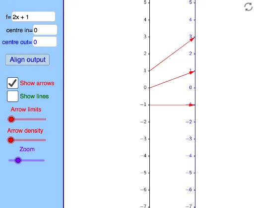
可调节输出中心的映射图
几何画板及绘图内容加载中,请稍等……
①这个范例演示了如何使用映射图代替传统图像来表示函数;②涉及的核心数学概念包括函数表示、映射关系、几何直观;③作图要点提炼自构造摘要,使用了TableText, Corner, Distance, Line, Text, panelleft1, Textfield, If, Sequence, Vector, Zip等GeoGebra命令/对象;④适合高中数学教学,用于理解函数的不同表示方式及动态变化。
GeoGebra 命令及参数
TableText({{"0"}, {"\ \ \ \ \ \ \ \ \ \ \ \ \ \ \ \ "}}, "hc") → Xt0Corner(1) → corner1Corner(2) → corner2Corner(3) → corner3Corner(4) → corner4Corner(5) → screenDimDistance(corner1, corner2) → distXDistance(corner1, corner4) → distYLine(OY, yAxis) → YaxisLineText("(x,y) = (" + (x(A)) + "," + (y(A)) + ") in black coordinate system") → text2Text("(X,Y) = (" + (x(A) - x(OY)) + "," + (y(A) - y(OY)) + ") in blue coordinate system") → text1panelleft1(panelsize) → panelquad, panelseg1, panelseg2, panelseg3, panelseg4, panellineTextfield(f) → InputBox1Line(OX, yAxis) → XaxisLineTextfield(x0) → InputBox2If(minstepfrac > lg(5), 10^(minsteppower + 1), If[minstepfrac > lg(2), (5 * 10^(minsteppower)), If[minstepfrac > 0, (2 * 10^(minsteppower)), 10^(minsteppower)]]) → stepsizeSequence(Text[TableText[{{"\phantom{(}" + (x0 + (n * stepsize)) + ""}, {"\phantom{(} \ \ \ \ \ \ \ \ \ \ \ \ \ \ \ "}}, "hr"], (x(OX) - Distance[Corner[Xt0, 1], Corner[Xt0, 2]] + 7 / unitX, (n * steplength) + y(OX) + (Distance[Corner[Xt0, 1], Corner[Xt0, 4]] * 0.25) + 4 / unitY), true, true], n, ceil((y(Corner[1]) - y(OX)) / steplength), floor((y(Corner[4]) - y(OX)) / steplength)) → XaxisNumbersSequence(Segment[(x(OX), y(OX) + (n * steplength)), (x(OX) - 2 / unitX, y(OX) + (n * steplength))], n, ceil((y(Corner[1]) - y(OX)) / steplength), floor((y(Corner[4]) - y(OX)) / steplength)) → XaxisTicksSequence(Text[TableText[{{"\phantom{(}" + (y0 + (n * stepsize)) + ""}, {"\phantom{(} \ \ \ \ \ \ \ \ \ \ \ \ \ \ \ "}}, "hr"], (x(OY) - Distance[Corner[Xt0, 1], Corner[Xt0, 2]] + 7 / unitX, (n * steplength) + y(OY) + (Distance[Corner[Xt0, 1], Corner[Xt0, 4]] * 0.25) + 4 / unitY), true, true], n, ceil((y(Corner[1]) - y(OY)) / steplength), floor((y(Corner[4]) - y(OY)) / steplength)) → YaxisNumbersSequence(Segment[(x(OY), y(OY) + (n * steplength)), (x(OY) - 2 / unitX, y(OY) + (n * steplength))], n, ceil((y(Corner[1]) - y(OY)) / steplength), floor((y(Corner[4]) - y(OY)) / steplength)) → YaxisTicksVector((xpos, 0), (ypos, 0)) → uSequence(i / spacing, i, ((-numarrows) * spacing), (numarrows * spacing)) → arrowstartsZip(x0 + (as * numminstep), as, arrowstarts) → arrowxvalsZip(f(ax), ax, arrowxvals) → arrowyvalsZip((xpos, ((xv - x0) * steplength / stepsize)), xv, arrowxvals) → arrowxcoordsZip((ypos, ((yv - y0) * steplength / stepsize)), yv, arrowyvals) → arrowycoordsZip(Vector[ax, ay], ax, arrowxcoords, ay, arrowycoords) → arrowsZip(Line[ax, ay], ax, arrowxcoords, ay, arrowycoords) → linesTextfield(y0) → InputBox3Vector((xpos, 0), (ypos, ((f(x0) - y0) * steplength / stepsize))) → v
AI 绘图提示语参考
画一个函数的可视化映射图,包含两个坐标系,一个黑色坐标系和一个蓝色坐标系。在黑色坐标系中显示一个点 (x,y),并在蓝色坐标系中显示对应的点 (X,Y)。在 x 轴和 y 轴上按一定步长标注刻度,并用箭头连接每个 x 值和其对应的函数值 y,箭头起点在 x 轴上,终点在 y 轴上,颜色区分输入和输出。整个图形应清晰展示函数的映射关系。
以上提示语为根据原始绘图命令整理而来,仅供参考。