
Lotka-Volterra 模型
几何画板及绘图内容加载中,请稍等……
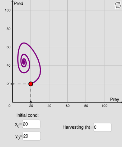
①本范例演示了捕食者-被捕食者动态系统的周期性种群数量变化图形;②涉及的核心数学概念为微分方程、函数图像、连续性;③作图要点:使用了 SolveODE, Length, First, Sequence, Element, Distance, Textfield, Ray, Text, NSolveODE, Point, Last, If, Segment, Polygon, Centroid 等GeoGebra命令与对象;④适合高中及以上学生及需要理解生态数学模型的用户。
GeoGebra 命令及参数
SolveODE(g, f, x(A), y(A), time, step) → numericalIntegral1Length(numericalIntegral1) → len01First(numericalIntegral1, len01) → list1Sequence((floor((step * i)), x(Element[list1, i])), i, 1, len01) → listpreyElement(listprey, explore) → preyPointSequence((floor((step * i)), y(Element[list1, i])), i, 1, len01) → listpredatorElement(listpredator, explore) → predPointElement(list1, position) → BDistance(B, P2) → CondTextfield(x_0) → InputBox1Textfield(y_0) → InputBox2Textfield(h) → InputBox3Ray(timePoint, predPoint) → iText(("Pred=" * y(predPoint))) → textpreyText(("Prey=" * y(preyPoint))) → textpredNSolveODE({f1, g1}, 0, {x_0, y_0}, time) → numericalIntegral2, numericalIntegral2_2Point(numericalIntegral1) → CLast(listpredator) → LastpredatorElement(Lastpredator, 1) → MMIf(MM ≟ MM, MM, (1 / 2, 1 / 2)) → MMMSegment(D, C') → kSegment(E, C') → jPolygon(F, G, 5) → poly1, l, m, n, p, q, H, I, JCentroid(poly1) → K