
逻辑斯蒂映射的 cobweb 图与李雅普诺夫指数
几何画板及绘图内容加载中,请稍等……
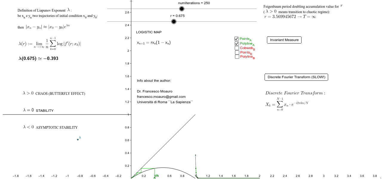
①本范例演示了逻辑斯蒂映射的 cobweb 图及其李雅普诺夫指数的计算与可视化;②涉及的核心数学概念包括逻辑斯蒂映射、迭代序列、李雅普诺夫指数、傅里叶变换;③作图要点:使用了 Point, IterationList, Segment, Sequence, PolyLine 等命令,以及 numIterations, N, r, f, values, λ 等对象;④适合高中及以上数学学习者,用于理解混沌理论与动力系统。
GeoGebra 命令及参数
Point(xAxis) → AIterationList(f, x(A), numIterations) → valuesPoint(xAxis) → BSegment(A, (x(A), f(x(A)))) → bSequence(Segment[(Element[values, i], Element[values, i + 1]), (Element[values, i + 1], Element[values, i + 1])], i, 1, numIterations - 1) → cobwebHorizontalSequence(Segment[(Element[values, i], Element[values, i]), (Element[values, i], Element[values, i + 1])], i, 2, numIterations) → cobwebVerticalIterationList(f, x(B), numIterations) → valuesBSegment(B, (x(B), f(x(B)))) → cSequence(Segment[(Element[valuesB, i], Element[valuesB, i + 1]), (Element[valuesB, i + 1], Element[valuesB, i + 1])], i, 1, numIterations - 1) → cobwebHorizontalBSequence(Segment[(Element[valuesB, i], Element[valuesB, i]), (Element[valuesB, i], Element[valuesB, i + 1])], i, 2, numIterations) → cobwebVerticalBSequence((1 + i / numIterations, Element[values, i]), i, 1, numIterations) → SERIEverdeSequence((1 + i / numIterations, Element[valuesB, i]), i, 1, numIterations) → SERIErossaPolyLine(SERIEverde) → verdePolyLine(SERIErossa) → rossaPoint({-1 + r / 4, Liap + 1}) → λPoint({0, r}) → f1Point({0.5, 0}) → f2Point({1, r}) → f3PolyLine(f1, f2, f3) → assDERIVATASegment((0, 0), (1, 1)) → mSegment((-2, 1), (0, 1)) → dSequence(i / Barre, i, 0, Barre) → CLASSBOUND
AI 绘图提示语参考
画一个Logistic Map的蛛网图,展示迭代序列的轨迹,并用不同颜色的折线表示正向和反向的迭代路径。同时,计算并可视化Liapunov指数,在图中标出关键点,并绘制导数函数的图像以及一条对角线,最后用不同颜色的条形图表示概率分布。
以上提示语为根据原始绘图命令整理而来,仅供参考。