
线性回归:拖拽点或输入数据拟合直线
几何画板及绘图内容加载中,请稍等……
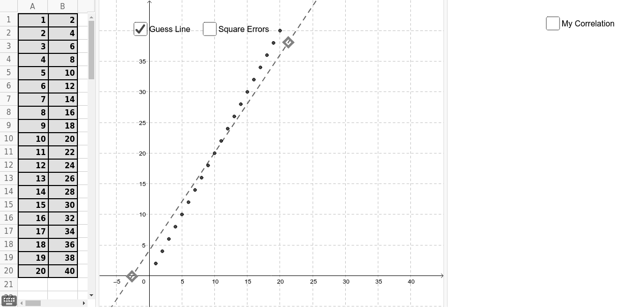
① 本范例演示了如何通过用户自定义数据点(拖拽或表格输入)进行线性回归,并直观展示拟合直线与数据点的关系。② 核心数学概念包括最小二乘法线性回归、残差、决定系数(R²)、样本标准差、中位数等统计量,以及直线方程与交点。③ 作图要点:使用GeoGebra的FitLineY命令计算回归直线,Line命令绘制直线,Intersect求交点,Polygon和Vector辅助展示数据范围或残差向量,RSquare和SampleSD计算统计指标,Text显示结果,Circle可能用于绘制置信区间或误差圆,数据点通过表格对象(A1-A20等)和列表list_x管理。④ 适合高中至大学阶段的统计与数据分析教学,也可用于数学实验课,帮助学生理解回归分析的本质和参数含义。
GeoGebra 命令及参数
Line(U, V) → line_{guess}Line(A, x = 0) → aLine(B, x = 0) → bLine(C, x = 0) → cLine(D, x = 0) → dLine(E, x = 0) → eLine(F, x = 0) → fLine(G, x = 0) → gLine(H, x = 0) → hLine(I, x = 0) → iLine(J, x = 0) → jLine(K, x = 0) → kLine(L, x = 0) → lLine(M, x = 0) → mLine(N, x = 0) → nLine(NP, x = 0) → npLine(O, x = 0) → pLine(P, x = 0) → qLine(R, x = 0) → sLine(S, x = 0) → tIntersect(line_{guess}, a) → A'Intersect(line_{guess}, b) → B'Intersect(line_{guess}, c) → C'Intersect(line_{guess}, d) → D'Intersect(line_{guess}, e) → E'Intersect(line_{guess}, f) → F'Intersect(line_{guess}, g) → G'Intersect(line_{guess}, h) → H'Intersect(line_{guess}, i) → I'Intersect(line_{guess}, j) → J'Intersect(line_{guess}, k) → K'Intersect(line_{guess}, l) → L'Intersect(line_{guess}, m) → M'Intersect(line_{guess}, n) → N'Intersect(line_{guess}, np) → NP'Intersect(line_{guess}, p) → O'Intersect(line_{guess}, q) → P'Intersect(line_{guess}, s) → R'Intersect(line_{guess}, t) → S'Line(Q, x = 0) → rIntersect(line_{guess}, r) → Q'Polygon(A', A, 4) → poly1, a_1, b_1, c_1, d_1, T, WPolygon(B', B, 4) → poly2, e_1, f_1, g_1, h_1, Z, A_1Polygon(D', D, 4) → poly3, i_1, j_1, k_1, l_1, B_1, C_1Polygon(E', E, 4) → poly4, m_1, n_1, p_1, q_1, D_1, E_1Polygon(C', C, 4) → poly5, r_1, s_1, t_1, a_2, F_1, G_1Polygon(F', F, 4) → poly6, b_2, c_2, d_2, e_2, H_1, I_1Polygon(G', G, 4) → poly7, f_2, g_2, h_2, i_2, J_1, K_1Polygon(H', H, 4) → poly8, j_2, k_2, l_2, m_2, L_1, M_1Polygon(I', I, 4) → poly9, n_2, p_2, q_2, r_2, N_1, O_1Polygon(J', J, 4) → poly10, s_2, t_2, a_3, b_3, P_1, Q_1Polygon(K', K, 4) → poly11, c_3, d_3, e_3, f_3, R_1, S_1Polygon(L', L, 4) → poly12, g_3, h_3, i_3, j_3, T_1, U_1Polygon(M', M, 4) → poly13, k_3, l_3, m_3, n_3, V_1, W_1Polygon(N', N, 4) → poly14, p_3, q_3, r_3, s_3, Z_1, A_2Polygon(NP', NP, 4) → poly15, t_3, a_4, b_4, c_4, B_2, C_2Polygon(P', P, 4) → poly16, d_4, e_4, f_4, g_4, D_2, E_2Polygon(O', O, 4) → poly17, h_4, i_4, j_4, k_4, F_2, G_2Polygon(Q', Q, 4) → poly18, l_4, m_4, n_4, p_4, H_2, I_2Polygon(R', R, 4) → poly19, q_4, r_4, s_4, t_4, J_2, K_2Polygon(S', S, 4) → poly20, a_5, b_5, c_5, d_5, L_2, M_2Vector((x(A), 0), (x(A), y(A) - y(A'))) → V_AVector((x(B), 0), (x(B), y(B) - y(B'))) → V_BVector((x(C), 0), (x(C), y(C) - y(C'))) → V_CVector((x(D), 0), (x(D), y(D) - y(D'))) → V_DVector((x(E), 0), (x(E), y(E) - y(E'))) → V_EVector((x(F), 0), (x(F), y(F) - y(F'))) → V_FVector((x(G), 0), (x(G), y(G) - y(G'))) → V_GVector((x(H), 0), (x(H), y(H) - y(H'))) → V_HVector((x(I), 0), (x(I), y(I) - y(I'))) → V_IVector((x(J), 0), (x(J), y(J) - y(J'))) → V_JVector((x(K), 0), (x(K), y(K) - y(K'))) → V_KVector((x(L), 0), (x(L), y(L) - y(L'))) → V_LVector((x(M), 0), (x(M), y(M) - y(M'))) → V_MVector((x(N), 0), (x(N), y(N) - y(N'))) → V_NVector((x(NP), 0), (x(NP), y(NP) - y(NP'))) → V_{NP}Vector((x(P), 0), (x(P), y(P) - y(P'))) → V_PVector((x(Q), 0), (x(Q), y(Q) - y(Q'))) → V_QVector((x(R), 0), (x(R), y(R) - y(R'))) → V_RVector((x(O), 0), (x(O), y(O) - y(O'))) → V_OVector((x(S), 0), (x(S), y(S) - y(S'))) → V_SRSquare(data, line_{guess}) → StrengthSampleSD(list_y) → SD_yMedian(list_x) → Median_xVector((Median_x / 2, (SD_y * 2)), (Median_x / 2, (SD_y * 2) + over)) → Vector_{over}Vector((Median_x / 2, (SD_y * 2)), (Median_x / 2, (SD_y * 2) - under)) → Vector_{under}Text(((Strength * 100) * "%"), ((Median_x * 1.425), (SD_y * 1.95))) → text1FitLineY(data) → line_{actual}Circle(((Median_x * 1.5), (2 * SD_y)), (Strength * Max[list_y] / 6)) → g_5Circle(((Median_x * 1.5), (2 * SD_y)), (Strength * Max[list_y] / 6)) → CorrelationCircleCircle(((Median_x * 1.5), (2 * SD_y)), (Strength * Max[list_y] / 6)) → CorrelationCircle_1Circle(((Median_x * 1.5), (2 * SD_y)), (Strength * Max[list_y] / 6)) → f_5
AI 绘图提示语参考
绘制一组散点数据点,每个点通过垂直线连接到一条可拖动的拟合直线上,形成残差矩形。拟合直线由两个可移动点确定,数据点可在表格中编辑。显示拟合直线的方程、决定系数、样本标准差等统计信息,并用不同颜色区分残差矩形。
以上提示语为根据原始绘图命令整理而来,仅供参考。