
指数函数y=kax的图像绘制
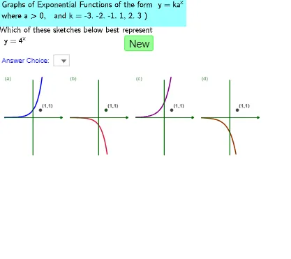
几何画板及绘图内容加载中,请稍等……
本范例演示如何绘制指数函数y=kax的图像。核心数学概念包括指数函数的性质和图像特征。通过使用GeoGebra命令如Simplify、Shuffle等,可以动态调整参数k和a,观察图像的变化。适合高中数学教学和学习。
GeoGebra 命令及参数
Simplify((RandomElement[liste_a]^(x) * Element[liste_k, 1])) → F12Simplify((RandomElement[liste_a]^(x) * Element[liste_k, 3])) → F11Simplify((RandomElement[liste_a]^(x) * Element[liste_k, 2])) → F10Simplify((RandomElement[liste_a]^(x) * Element[liste_k, 1])) → F9Shuffle({9, 11, 13, 15}) → listshowGf1, {13, 11, 15, 9}Shuffle({10, 12, 14, 16}) → listshowGf2, {16, 14, 12, 10}Shuffle({9, 10, 13, 14}) → listshowGf3, {9, 14, 13, 10}Shuffle({11, 12, 15, 16}) → listshowGf4, {16, 15, 11, 12}Shuffle({9, 12, 13, 16}) → listshowGf5, {13, 9, 12, 16}Shuffle({10, 11, 14, 15}) → listshowGf6, {14, 11, 10, 15}Sequence(If[count < 3, Element[listshowGf0, i], If[count < 5, Element[listshowGf1, i], If[count < 7, Element[listshowGf2, i], If[count < 9, Element[listshowGf3, i], If[count < 11, Element[listshowGf4, i], If[count < 11, Element[listshowGf5, i], Element[listshowGf6, i]]]]]]], i, 1, 4) → listnsGIf(useG, If[count > 2, Random[0, 7], 3], Random[0, 7]) → e'Random(1, 4) → dIf(count > 2, Random[1, 4], If[count > 1, 3, 1]) → n_gIf(d ≟ e' ∧ (count > 8 ∨ count < 5), 1, e') → eRandom(1, 4) → n_fShuffle({1, 2, 3, 4}) → listshowFf1, {4, 1, 3, 2}Shuffle({1, 4, 5, 8}) → listshowFf2a, {1, 8, 4, 5}Shuffle({2, 3, 6, 7}) → listshowFf2b, {6, 2, 3, 7}If(count < 5, Element[listFf, Element[listshowFf1, 3]], If[count < 9, Element[listFf, Element[listshowFf2a, 3]], Element[listFf, Element[listshowFf2b, 3]]]) → f_{3s}Coefficients(f_{3s}) → listf_{3s}If(count < 5, Element[listFf, Element[listshowFf1, 4]], If[count < 9, Element[listFf, Element[listshowFf2a, 4]], Element[listFf, Element[listshowFf2b, 4]]]) → f_{4s}Coefficients(f_{4s}) → listf_{4s}If(count < 5, Element[listFf, Element[listshowFf1, 1]], If[count < 9, Element[listFf, Element[listshowFf2a, 1]], Element[listFf, Element[listshowFf2b, 1]]]) → f_{1s}Coefficients(f_{1s}) → listf_{1s}If(count < 5, Element[listFf, Element[listshowFf1, 2]], If[count < 9, Element[listFf, Element[listshowFf2a, 2]], Element[listFf, Element[listshowFf2b, 2]]]) → f_{2s}Coefficients(f_{2s}) → listf_{2s}Element(listCoeffs, n_f, 1) → a_fElement(listCoeffs, n_f, 2) → b_fSimplify((-F9(x))) → F13Simplify((-F10(x))) → F14Simplify((-F11(x))) → F15Simplify((-F12(x))) → F16Sequence(Sequence[(x(A) + (s_p * i), y(A) + (s_p * j)), i, 0, 3], j, 0, 0) → list3CtrofGraphs, {{(5, 0), (13.8, 0), (22.6, 0), (31.400000000000002, 0)}}Polygon(E, D, F, G) → poly2, e_1, d_1, f_5, gPolygon(J, K, L, M) → poly4, j, k, l, mPolygon(J, K, C, B) → poly5, j_1, k_1, c, b_1Sequence(Sequence[Segment[(x(A) + (s_p * i) - l_x / 2, y(A) + (s_p * j)), (x(A) + (s_p * i) + l_x / 2, y(A) + (s_p * j))], i, 0, 3], j, 0, 0) → list1Xaxes, {{7.6000000000000005, 7.600000000000001, 7.600000000000001, 7.600000000000001}}Sequence(Sequence[Segment[(x(A) + (s_p * i), y(A) + (s_p * j) - l_y / 2), (x(A) + (s_p * i), y(A) + (s_p * j) + l_y / 2)], i, 0, 3], j, 0, 0) → list2Yaxes, {{10, 10, 10, 10}}Sequence(Sequence[(x(A) + l_x / 2 + (s_p * i), y(A) + (s_p * j)), i, 0, 3], j, 0, 0) → listXarrow, {{(8.8, 0), (17.6, 0), (26.400000000000002, 0), (35.2, 0)}}Sequence(Sequence[Text[Element[listChoicestext, i + 1], (x(A) - l_x / 2 + (s_p * (i - 1)), y(A) + l_y / 2)], i, 1, 4], j, 0, 0) → listChoicestextDisplay, {{"(a)", "(b)", "(c)", "(d)"}}Element(listCoeffs, n_f, 3) → c_fIf(useG, x(Element[listTurningPointsG, Element[listnsG, n_g] - 8]), ((-b_f)) / ((2 * a_f))) → symx2Defined(root1) → realrootsIf(count < 5, Element[listFf, Element[listshowFf1, 4]], If[count < 9, Element[listFf, Element[listshowFf2a, 4]], Element[listFf, Element[listshowFf2b, 4]]]) → f_{tests}Polygon(B, C, D, E) → poly1, b, c_1, d_2, e_2If(count < 5, Element[listshowFf1, n_f], If[count < 9, Element[listshowFf2a, n_f], Element[listshowFf2b, n_f]]) → n_sSequence(If[count < 5, Element[listshowFf1, i], If[count < 9, Element[listshowFf2a, i], Element[listshowFf2b, i]]], i, 1, 4) → listnsFMin(d, e) → I1Min((-d), e) → I2Min(d, (-e)) → I3Min((-d), (-e)) → I4Min(d, e) → I5Min((-d), e) → I6Min(d, (-e)) → I7Min((-d), (-e)) → I8Max(d, e) → J1Max((-d), e) → J2Max((-d), e) → J6Max(d, (-e)) → J7Max(d, (-e)) → J3Max((-d), (-e)) → J4Max(d, e) → J5Max((-d), (-e)) → J8Element(listGf, Element[listnsG, 1] - 8) → g_{1s}Element(listGf, Element[listnsG, 2] - 8) → g_{2s}Element(listGf, Element[listnsG, 4] - 8) → g_{4s}Element(listGf, Element[listnsG, 3] - 8) → g_{3s}Sequence((0, Cell[7, 8 + i]), i, 1, 8) → listyinterceptsElement(Coefficients[Simplify[Cell[6, Element[listnsG, n_g]]]], 2) → b_gElement(Coefficients[Simplify[Cell[6, Element[listnsG, n_g]]]], 3) → c_gElement(Coefficients[Simplify[Cell[6, Element[listnsG, n_g]]]], 1) → a_gIntersect(f_{1one}, f_{12minusx}) → N
AI 绘图提示语参考
绘制指数函数 y = k a^x 的图像,展示参数 k 和 a 变化对函数图像的影响。首先画出三条不同的指数函数图像,每条使用不同的 k 值和 a 值。然后在坐标系中添加 x 轴和 y 轴,并在 x 轴上标注 (a)、(b)、(c)、(d) 标签。最后,根据函数的系数绘制图像的对称轴和顶点,并标注关键点。
以上提示语为根据原始绘图命令整理而来,仅供参考。