
向量场穿过线段的通量可视化
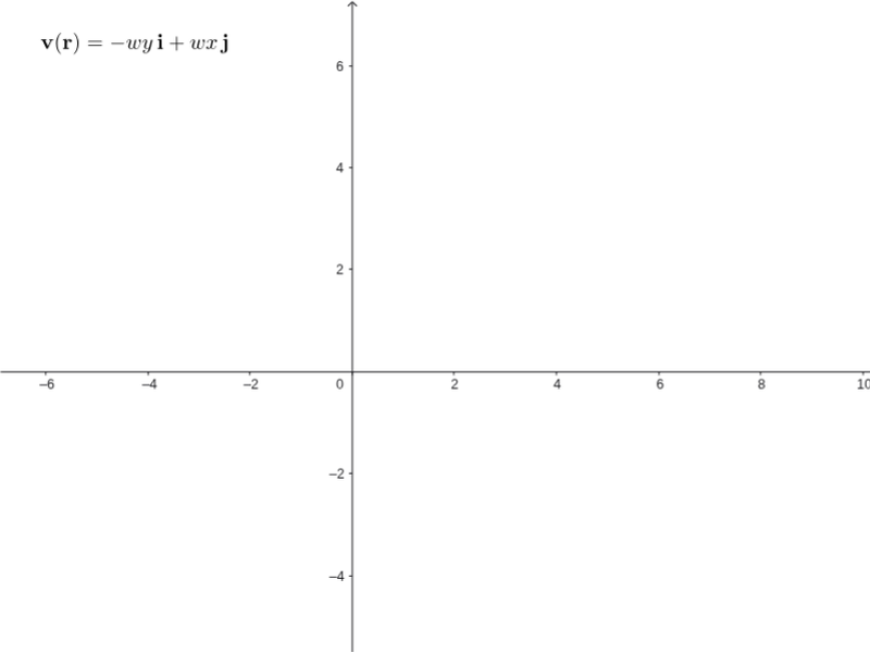
几何画板及绘图内容加载中,请稍等……
该范例演示了向量场穿过一条线段的通量(Flux)的几何与数值计算。核心数学概念是向量场的通量,即向量场与线段法向量的点积沿线段长度的积分,它衡量了场穿过该线段的净流量。作图要点:使用GeoGebra的Sequence生成粒子序列,Circle绘制标记,Derivative和Integral计算导数与积分,CurveCartesian定义向量场曲线,Segment构造线段,Midpoint和Translate辅助定位,同时通过滑块(如a、b)和网格(grid、scale)控制参数与显示。适合大学微积分或多元微积分课程中讲解线积分与通量概念,也可用于高中进阶物理中场的可视化教学。
GeoGebra 命令及参数
Sequence(Sequence[Vector[(j, k), (j + (scale * F_1(j, k)), k + (scale * F_2(j, k)))], j, xmin, xmax, xstep], k, ymin, ymax, ystep) → vField, {{(1.3358585902573044, -1.3856264649362657), (1.3358585902573044, -1.039496479841132), (1.3358585902573044, -0.693366494745999), (1.3358585902573044, -0.34723650965086517), (1.3358585902573044, -0.0011065245557322356), (1.3358585902573041, 0.3450234605394016), (1.3358585902573044, 0.6911534456345345), (1.3358585902573044, 1.0372834307296674), (1.3358585902573044, 1.3834134158248013)}, {(1.0043951299543386, -1.3856264649362657), (1.0043951299543377, -1.039496479841132), (1.004395129954338, -0.693366494745999), (1.004395129954338, -0.34723650965086517), (1.004395129954338, -0.0011065245557322356), (1.0043951299543383, 0.3450234605394016), (1.0043951299543377, 0.6911534456345345), (1.0043951299543386, 1.0372834307296674), (1.0043951299543377, 1.3834134158248013)}, {(0.6729316696513719, -1.3856264649362657), (0.6729316696513719, -1.039496479841132), (0.6729316696513719, -0.693366494745999), (0.6729316696513716, -0.34723650965086517), (0.6729316696513717, -0.0011065245557322356), (0.6729316696513716, 0.34502346053940114), (0.6729316696513719, 0.6911534456345345), (0.6729316696513719, 1.0372834307296674), (0.6729316696513719, 1.383413415824801)}, {(0.34146820934840516, -1.3856264649362653), (0.34146820934840516, -1.039496479841132), (0.34146820934840516, -0.6933664947459985), (0.3414682093484054, -0.34723650965086517), (0.3414682093484054, -0.0011065245557322356), (0.3414682093484054, 0.34502346053940114), (0.34146820934840516, 0.6911534456345345), (0.34146820934840516, 1.0372834307296677), (0.34146820934840516, 1.383413415824801)}, {(0.010004749045439354, -1.3856264649362653), (0.010004749045439354, -1.039496479841132), (0.01000474904543891, -0.6933664947459987), (0.01000474904543891, -0.3472365096508654), (0.010004749045439, -0.0011065245557321454), (0.01000474904543891, 0.34502346053940114), (0.01000474904543891, 0.6911534456345344), (0.010004749045439354, 1.0372834307296677), (0.010004749045439354, 1.383413415824801)}, {(-0.32145871125752734, -1.3856264649362653), (-0.32145871125752734, -1.039496479841132), (-0.32145871125752734, -0.6933664947459987), (-0.3214587112575271, -0.3472365096508654), (-0.32145871125752734, -0.0011065245557322356), (-0.32145871125752734, 0.34502346053940114), (-0.32145871125752734, 0.6911534456345345), (-0.32145871125752734, 1.0372834307296674), (-0.32145871125752734, 1.3834134158248013)}, {(-0.652922171560494, -1.3856264649362653), (-0.652922171560494, -1.039496479841132), (-0.652922171560494, -0.6933664947459985), (-0.6529221715604938, -0.34723650965086517), (-0.6529221715604937, -0.0011065245557322356), (-0.6529221715604938, 0.34502346053940114), (-0.6529221715604936, 0.6911534456345345), (-0.652922171560494, 1.0372834307296674), (-0.652922171560494, 1.3834134158248013)}, {(-0.9843856318634598, -1.3856264649362653), (-0.9843856318634598, -1.039496479841132), (-0.9843856318634598, -0.693366494745999), (-0.9843856318634601, -0.34723650965086517), (-0.9843856318634601, -0.0011065245557322356), (-0.9843856318634601, 0.3450234605394016), (-0.9843856318634598, 0.6911534456345345), (-0.9843856318634598, 1.0372834307296674), (-0.9843856318634598, 1.3834134158248013)}, {(-1.3158490921664265, -1.3856264649362657), (-1.3158490921664265, -1.039496479841132), (-1.3158490921664265, -0.693366494745999), (-1.3158490921664263, -0.34723650965086517), (-1.3158490921664265, -0.0011065245557322356), (-1.3158490921664265, 0.3450234605394016), (-1.3158490921664265, 0.6911534456345345), (-1.3158490921664265, 1.0372834307296674), (-1.3158490921664265, 1.3834134158248013)}}Sequence(((x(Element[inicialPts, i]) * cos((w * time))) - (y(Element[inicialPts, i]) * sin((w * time))), (x(Element[inicialPts, i]) * sin((w * time))) + (y(Element[inicialPts, i]) * cos((w * time)))), i, 1, 8) → particlesListSequence(CurveCartesian[(x(Element[inicialPts, i]) * cos((w * t))) - (y(Element[inicialPts, i]) * sin((w * t))), (x(Element[inicialPts, i]) * sin((w * t))) + (y(Element[inicialPts, i]) * cos((w * t))), t, 0, time], i, 1, 8) → pathlinesListCircle(divPt, 0.5) → divGlowCircleSequence(Segment[Rotate[curlPt - (0.5, 0), k + curlAngle, curlPt], Rotate[curlPt + (0.5, 0), k + curlAngle, curlPt]], k, 0, 2.0944, 1.0472) → spokesDerivative(Curve_x) → dCurve_xDerivative(Curve_y) → dCurve_ySimplify(Pdy(x) - Qdx(x)) → fIntegral(f, 0, t) → FluxCurveCartesian((Curve_x(u), Curve_y(u)), u, 0, 1) → pathCurveCartesian((Curve_x(u), Curve_y(u)), u, 0, t) → parPathSegment(path(0.6), path(0.6 + 0.1)) → arrow2Segment(path(0.3), path(0.3 + 0.1)) → arrow1Sequence(Vector[path(s), path(s) + ((scale * F_1(x(path(s)), y(path(s)))), (scale * F_2(x(path(s)), y(path(s)))))], s, 0, t, 0.1) → pathVectorsMidpoint(I, J) → MidPointTranslate(normalvector, MidPoint) → n
AI 绘图提示语参考
绘制一个向量场穿过线段的通量可视化图形。首先画出线段和向量场,向量场用多个箭头表示,线段用直线表示。接着在线段上生成多条路径线,展示向量场中粒子的运动轨迹。在线段上标出法向量,并用箭头表示向量场在该点的方向。最后,计算并显示向量场穿过线段的通量,用颜色或数值表示通量的大小。
以上提示语为根据原始绘图命令整理而来,仅供参考。