
配方法几何可视化:完全平方公式的GeoGebra动态演示
几何画板及绘图内容加载中,请稍等……
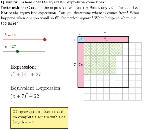
本范例通过GeoGebra动态演示配方法(Completing the Square)的几何意义,将抽象的代数运算转化为直观的面积填充问题。核心数学概念包括完全平方公式、二次方程的一般形式与顶点式转换、配方法的几何解释。作图要点:利用LaTeX命令动态显示代数表达式演变过程,使用Polygon绘制正方形和多边形来可视化“补全”平方的操作,通过Sequence自动生成水平线和垂直线网格,A1、A2、A3等对象构建分步演示流程,配合TryAnother、Initialize等交互元素实现个性化练习。适合中学八年级及以上学生理解配方法的原理,或作为教师课堂演示二次方程求解技巧的辅助工具。
GeoGebra 命令及参数
LaTeX((((("\text{" * QUESTION) * "\\") * INSTRUCTIONS) * "}")) → TEXTLaTeX(("b=" * b)) → bLabelLaTeX(("c=" * c)) → cLabelSequence(Segment[Point[{1, j}], Point[{10, j}]], j, -10, -1) → horizontalLinesSequence(Segment[Point[{k, -1}], Point[{k, -10}]], k, 1, 10) → verticalLinesPolygon({(0, 0), (1, 0), (1, -1), (0, -1)}) → A1Polygon((1, -1 - floorRootC), (1 + floorRootC, -1 - floorRootC), 4) → A4aPolygon({(0, 0), (1, 0), (1, -1), (0, -1)}) → A1borderPolygon({(1, 0), (1 + halfB, 0), (1 + halfB, -1), (1, -1)}) → A2Polygon({(1, 0), (1 + halfB, 0), (1 + halfB, -1), (1, -1)}) → A2borderPolygon({(0, -1), (1, -1), (1, -1 - halfB), (0, -1 - halfB)}) → A3Polygon({(0, -1), (1, -1), (1, -1 - halfB), (0, -1 - halfB)}) → A3borderPolygon({(1 + floorRootC, -1), (1 + floorRootC + 1, -1), (1 + floorRootC + 1, -1 - Min[leftOverC, floorRootC]), (1 + floorRootC, -1 - Min[leftOverC, floorRootC])}) → A4bPolygon({(1, -1 - floorRootC), (1, -1 - floorRootC - 1), (1 + Max[leftOverC - floorRootC, 0], -1 - floorRootC - 1), (1 + Max[leftOverC - floorRootC, 0], -1 - floorRootC)}) → A4cPolygon({(0, 0), (halfB + 1, 0), (halfB + 1, (-(halfB + 1))), (0, (-(halfB + 1)))}) → fullSquareText("x^2", (0, 0), true, true) → labelAText((("\vphantom{x^2}" * If[halfB ≟ 1, "", "" + halfB]) * "x"), (1 + (halfB - 1) / 2, 0), true, true) → labelBText((("\vphantom{x^2}" * If[halfB ≟ 1, "", "" + halfB]) * "x"), (0, -1 - (halfB - 1) / 2), true, true) → labelCText("x", (0, 0.75), true, true) → labelDText(halfB, (1 + (halfB - 1) / 2, 0.75), true, true) → labelEText("\vphantom{x^2}x", (-0.75, 0), true, true) → labelFText(("\vphantom{x^2}" * halfB), (-0.75, -1 - (halfB - 1) / 2), true, true) → labelG
AI 绘图提示语参考
在坐标平面上绘制一个 10×10 的网格,横线从 y=-10 到 -1,纵线从 x=1 到 10;在原点处放一个单位正方形表示 x²,右侧和下方各加一个宽为 b/2 的长方形分别表示 (b/2)x;再在右下方拼补若干小矩形以填满常数项 c,使整体形成边长 1+b/2 的大正方形;在各图形上标注 x²、b/2 x、x 及对应数值,整体呈现配方法几何补全过程。
以上提示语为根据原始绘图命令整理而来,仅供参考。