Volumes of Revolution about the x-axis

Loading the math board and drawing, please wait…

2015-10-29 16:02

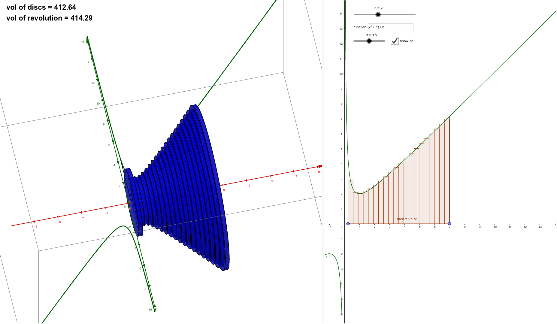
① This example demonstrates the solid generated by revolving a function graph around the x‑axis, visualizing the shape and the volume integration process. ② Core mathematical concepts include definite integrals, the volume‑of‑revolution formula, Riemann sum approximation, and the limit concept. ③ Construction highlights: Point, Sequence, Segment, RectangleSum, and Sum commands build discrete disc approximations; an InputBox controls the integration interval; objects such as discs, discswire, vol, and area dynamically display slices and accumulated volume. ④ Suitable for high‑school calculus electives, introductory university calculus courses, and self‑study, helping learners connect discrete summation to continuous integration.

GeoGebra Commands & Parameters

Point(xAxis) → B
Point(xAxis) → A
Sequence(i, i, x(A), x(B), (x(B) - x(A)) / n) → xval
Segment(A, C) → a
Segment(B, D) → b
Textfield(f) → InputBox1
Sequence(Cylinder[(Element[xval, i], 0), (Element[xval, i + 1], 0), f(((1 - d) * Element[xval, i]) + (d * Element[xval, i + 1]))], i, 1, n) → discs
Sum(discs) → vol
RectangleSum(f, x(A), x(B), n, d) → area
Sequence(Cylinder[(Element[xval, i], 0), (Element[xval, i + 1], 0), f(((1 - d) * Element[xval, i]) + (d * Element[xval, i + 1]))], i, 1, n) → discswire

AI Drawing Prompt Reference

This is a solid generated by revolving a function graph around the x-axis. The solid is approximated by a series of discrete discs, each corresponding to a subinterval of the function over the integration interval. The graphic also includes rectangle areas and summation processes to illustrate the approximation of volume. The overall shape is a rotation body, constructed through discrete approximations and summation.

The prompt above was compiled from the original drawing commands and is for reference only.