
Volume by Cylindrical Shells - Example: Torus
Loading the math board and drawing, please wait…
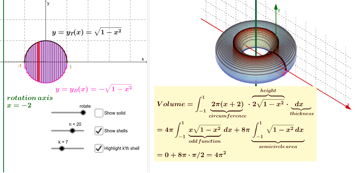
This example demonstrates the calculation of the volume of a torus using the method of cylindrical shells. Core mathematical concepts include integration, volume calculation, and the cylindrical shells method. The construction utilizes GeoGebra commands and objects such as Sequence, Surface, Polygon, and Segment to dynamically visualize the generation of the torus, providing an intuitive understanding of the geometric interpretation of integration. Suitable for high school and above students learning about volume calculation methods in calculus.
GeoGebra Commands & Parameters
Sequence(a + ((k - 0.5) * dx), k, 1, n) → midptsSequence(a + (k * dx), k, 0, n - 1) → leftptsSequence(a + (k * dx), k, 1, n) → rightptsSequence(Polygon[(xk(k - 1), y_B(Element[evalpts, k])), (xk(k - 1), y_T(Element[evalpts, k])), (xk(k), y_T(Element[evalpts, k])), (xk(k), y_B(Element[evalpts, k]))], k, 1, n) → RectanglesSequence((Element[evalpts, k], 0), k, 1, n) → evalptsplotSurface(xrot + ((xk(k - 1) - xrot) * cos(t)), h, ((xk(k - 1) - xrot) * sin(t)), t, 0, (2 * π), h, y_B(Element[evalpts, k]), y_T(Element[evalpts, k])) → ShellIn_kSurface(xrot + (r * cos(t)), y_T(Element[evalpts, k]), (r * sin(t)), t, 0, (2 * π), r, xk(k - 1) - xrot, xk(k) - xrot) → UpShell_kSurface(xrot + ((xk(k) - xrot) * cos(t)), h, ((xk(k) - xrot) * sin(t)), t, 0, (2 * π), h, y_B(Element[evalpts, k]), y_T(Element[evalpts, k])) → ShellOut_kSurface(xrot + (r * cos(t)), y_B(Element[evalpts, k]), (r * sin(t)), t, 0, (2 * π), r, xk(k - 1) - xrot, xk(k) - xrot) → ShellDown_kSequence(Surface[xrot + ((xk(k - 1) - xrot) * cos(t)), h, ((xk(k - 1) - xrot) * sin(t)), t, 0, (2 * π), h, y_B(Element[evalpts, k]), y_T(Element[evalpts, k])], k, 1, n) → ShellsInSequence(Surface[xrot + (r * cos(t)), y_T(Element[evalpts, k]), (r * sin(t)), t, 0, (2 * π), r, xk(k - 1) - xrot, xk(k) - xrot], k, 1, n) → ShellsUpSequence(Surface[xrot + (r * cos(t)), y_B(Element[evalpts, k]), (r * sin(t)), t, 0, (2 * π), r, xk(k - 1) - xrot, xk(k) - xrot], k, 1, n) → ShellsDownSequence(Surface[xrot + ((xk(k) - xrot) * cos(t)), h, ((xk(k) - xrot) * sin(t)), t, 0, (2 * π), h, y_B(Element[evalpts, k]), y_T(Element[evalpts, k])], k, 1, n) → ShellsOutSurface(xrot + (cos((-t)) * (u - xrot)), y_B(u), (sin((-t)) * (u - xrot)), u, a, b, t, 0, RotationAngle) → Solid_BSurface(xrot + (cos((-t)) * (u - xrot)), y_T(u), (sin((-t)) * (u - xrot)), u, a, b, t, 0, RotationAngle) → Solid_TSurface(xrot + ((a - xrot) * cos((-t))), h, ((a - xrot) * sin((-t))), t, 0, RotationAngle, h, y_B(a), y_T(a)) → Solid_aSurface(xrot + ((b - xrot) * cos((-t))), h, ((b - xrot) * sin((-t))), t, 0, RotationAngle, h, y_B(b), y_T(b)) → Solid_bSurface(xrot + (cos((-RotationAngle)) * (u - xrot)), ((1 - w) * y_B(u)) + (w * y_T(u)), (sin((-RotationAngle)) * (u - xrot)), w, 0, 1, u, a, b) → Solid_eSurface(xrot + u - xrot, ((1 - w) * y_B(u)) + (w * y_T(u)), (0 * (u - xrot)), w, 0, 1, u, a, b) → region3dPolygon((xk(k - 1), y_B(Element[evalpts, k])), (xk(k - 1), y_T(Element[evalpts, k])), (xk(k), y_T(Element[evalpts, k])), (xk(k), y_B(Element[evalpts, k]))) → Rectangle_k, f, g, h, iSegment((0, 0), (xrot, 0)) → c