Visualizing Finite and Infinite Limits

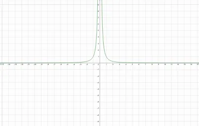
This example visualizes the approach behavior of a function for both finite limits and infinite limits, making it easier to see what happens as the independent variable approaches a point or grows without bound. It focuses on key calculus ideas: the distinction between limits that converge to a specific real value and limits that diverge to infinity (or negative infinity), along with the corresponding geometric behavior of the function’s graph near critical locations. Construction-wise, the GeoGebra model uses objects f, g, h, and p: f/g/h represent the relevant functions (curves or possibly 3D surfaces depending on the setup), while p serves as an auxiliary object to position the viewpoint/region and highlight the limit scenario. By coordinating these objects, the visualization emphasizes how the graph values change along the chosen approach, enabling a direct finite-vs-infinite comparison. Suitable for upper-secondary advanced study and early university calculus, especially for classroom demonstrations and conceptual review.