Visualizing and Constructing an Algebraic Surface

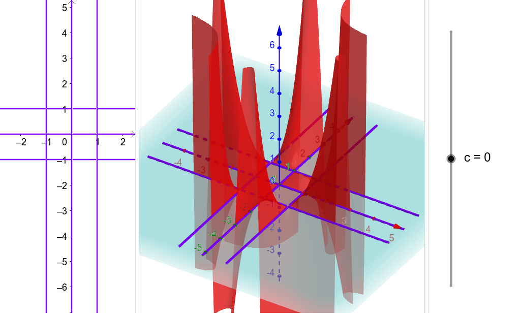
This GeoGebra example demonstrates the geometric construction and dynamic visualization of an algebraic surface in three-dimensional space, showing how implicit equations define complex spatial shapes. Core mathematical concepts include implicit surfaces, orthogonal cross-sections, and spatial implicit curves. To construct this, the example utilizes the `Surface` command to render the algebraic surface, integrated with `OrthogonalPlane` and `ImplicitCurve` commands to highlight intersections and cross-sectional profiles. Key parameters like `a`, `c`, `A`, `b`, and `d` are defined as adjustable objects, allowing users to manipulate the surface's geometry in real-time. This resource is ideal for university-level courses in advanced calculus, analytic geometry, algebraic geometry, or multivariable calculus, serving as a powerful tool for classroom instruction and self-study in 3D mathematical visualization.