
Unit Circle and Trigonometric Functions by Craig Cullen
Loading the math board and drawing, please wait…
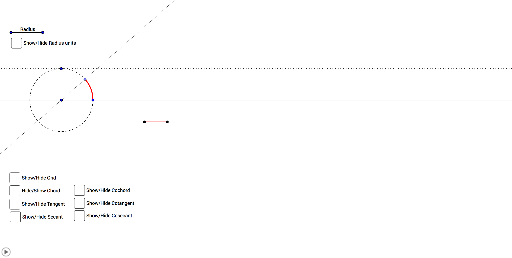
This example demonstrates the geometric interpretation of six trigonometric functions on a unit circle. It involves core concepts like the unit circle, trigonometric functions, geometric objects, angles, and arcs. The construction uses GeoGebra commands such as Vector, Translate, Ray, Point, Segment, Circle, CircleArc, Line, OrthogonalLine, Intersect, Rotate, and Mirror. It is suitable for high school mathematics education and learning, providing an intuitive understanding of the relationship between trigonometric functions and the unit circle.
GeoGebra Commands & Parameters
Vector((0, 0), (1, 0)) → vTranslate(A, v) → A'Ray(A, A') → aPoint(a) → BSegment(A, B) → bVector(A, B) → RadiusTranslate(C, Radius) → C'Circle(C, C') → cPoint(c) → DCircleArc(C, C', D) → dLine(C, C') → eOrthogonalLine(D, e) → fIntersect(f, e) → ESegment(D, E) → gPoint(Circle[F, abs(d)]) → GSegment(F, G) → hVector(E, D) → Chord_1OrthogonalLine(F, Radius) → iTranslate(i, Radius) → i'Translate(i', Radius) → i''Translate(i'', Radius) → i'''Translate(i''', Radius) → jTranslate(j, Radius) → j'Translate(j', Radius) → j''Translate(G, Chord_1) → G'Segment(G', G) → kIntersect(i', h) → HIntersect(i'', h) → IIntersect(i''', h) → JIntersect(j, h) → KIntersect(j', h) → LIntersect(j'', h) → MRotate(B, 90°, A) → B'Translate(A, Radius) → A'_1Vector(A, A'_1) → uVector(A, B') → wRay(F, G) → mTranslate(F, w) → F'Translate(G, w) → G'_1Ray(F', G'_1) → m'Translate(F', w) → F''Translate(G'_1, w) → NRay(F'', N) → m''Translate(F'', w) → F'''Translate(N, w) → N'Ray(F''', N') → m'''Mirror(F''', m) → OMirror(N', m) → N''Ray(O, N'') → nMirror(F'', m) → F'''_1Mirror(N, m) → N'_1Ray(F'''_1, N'_1) → m'''_1Mirror(F', m) → F''_1Mirror(G'_1, m) → PRay(F''_1, P) → m''_1OrthogonalLine(C', m') → lLine(C, D) → pIntersect(l, p) → QSegment(Q, C') → rVector(C', Q) → TangentTranslate(G, Tangent) → G'_2Segment(G'_2, G) → tIntersect(l, p) → RSegment(R, C) → a_1Point(a_1) → SVector(C, R) → SecantLine(C, C') → b_1OrthogonalLine(D, Secant) → c_1Intersect(b_1, c_1) → TVector(C, T) → Secant_2Translate(G, Secant_2) → G'_3Rotate(G'_3, 90°, G) → USegment(G, U) → d_1Segment(C, T) → e_1Ray(C, C') → g_1Rotate(C, 57.29577951308232°, C) → C'_1Rotate(C', 57.29577951308232°, C) → C''Ray(C'_1, C'') → h_1Intersect(d, h_1) → V,Rotate(C'_1, 57.29577951308232°, C) → WRotate(C'', 57.29577951308232°, C) → C'''Ray(W, C''') → i_1Rotate(W, 57.29577951308232°, C) → W'Rotate(C''', 57.29577951308232°, C) → ZRay(W', Z) → j_1Rotate(W', 57.29577951308232°, C) → W''Rotate(Z, 57.29577951308232°, C) → Z'Ray(W'', Z') → k_1Rotate(W'', 57.29577951308232°, C) → W'''Rotate(Z', 57.29577951308232°, C) → Z''Ray(W''', Z'') → l_1Rotate(W''', 57.29577951308232°, C) → A_1Rotate(Z'', 57.29577951308232°, C) → Z'''Ray(A_1, Z''') → m_1Intersect(d, i_1, 1) → B_1Intersect(d, j_1, 1) → C_1Intersect(d, k_1, 1) → D_1Intersect(d, l_1, 1) → E_1Intersect(d, m_1, 1) → F_1Line(D, b) → p_1OrthogonalLine(C, p_1) → q_1Intersect(p_1, q_1) → G_1Segment(D, G_1) → r_1Vector(G_1, D) → CochordTranslate(G, Cochord) → G'_4Rotate(G'_4, 90°, G) → H_1Segment(H_1, G) → s_1Rotate(C', 90°, C) → C''_1OrthogonalLine(C''_1, l) → t_1Intersect(p, t_1) → I_1Segment(C''_1, I_1) → a_2Vector(C''_1, I_1) → CotangentTranslate(G, Cotangent) → G'_5Rotate(G'_5, 90°, G) → J_1Segment(J_1, G) → b_2Line(C, C') → c_2Intersect(p, t_1) → K_1Segment(C, K_1) → d_2Line(C, C''_1) → e_2OrthogonalLine(D, d_2) → f_2Intersect(e_2, f_2) → L_1Segment(C, L_1) → g_2Vector(C, L_1) → CosecantTranslate(G, Cosecant) → G'_6Segment(G, G'_6) → h_2
AI Drawing Prompt Reference
Draw a unit circle and demonstrate the geometric interpretation of six trigonometric functions: sine, cosine, tangent, cotangent, secant, and cosecant. Start by drawing the unit circle, then draw a radius from point A to the center C. Next, take point B on the circle and draw a segment AB. Draw a ray from B to the positive x-axis, and take point D on the circle, drawing a circular arc CD. Draw a line perpendicular to the ray at point D, intersecting the x-axis at point E, and draw a segment DE. Construct the sine line, cosine line, tangent line, cotangent line, secant line, and cosecant line, and finally use reflection to obtain the secant and cosecant lines.
The prompt above was compiled from the original drawing commands and is for reference only.