
Three-Phase Circle: Representing Three-Phase Electricity Phases via Circular Mot
Loading the math board and drawing, please wait…
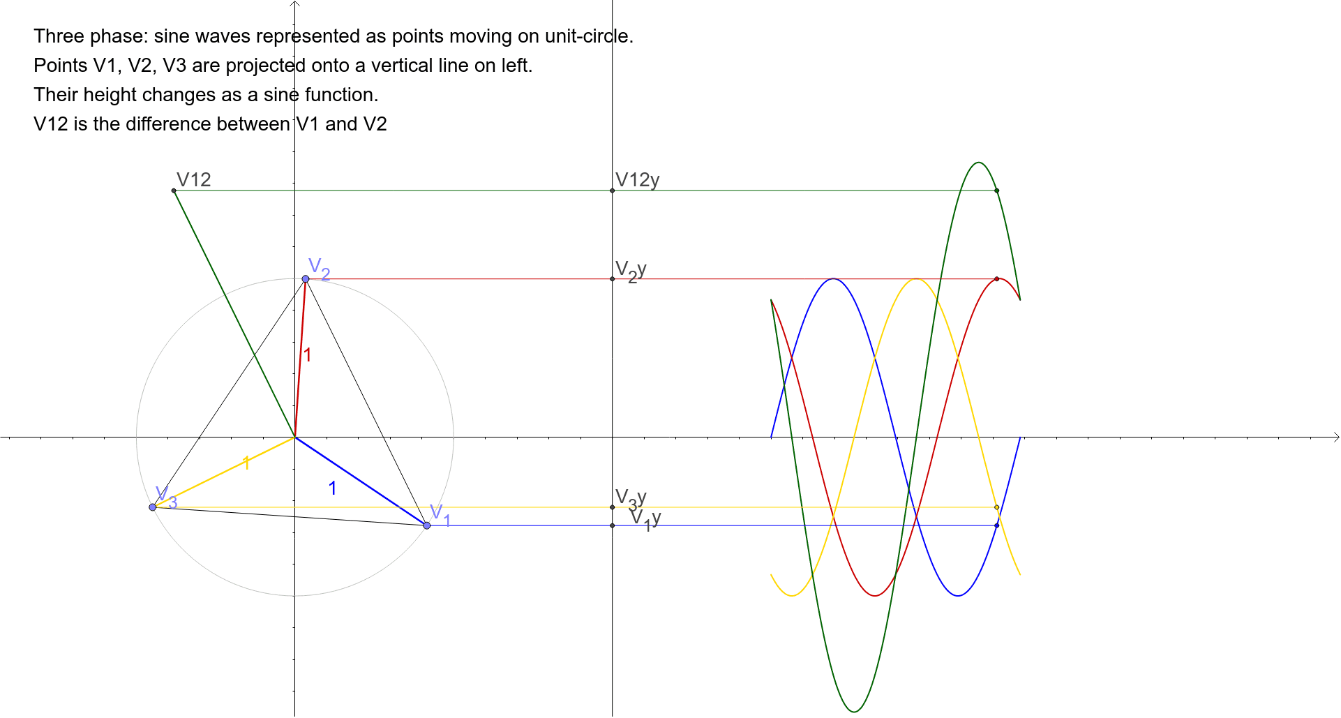
① This example demonstrates how the motion of points on a circle can represent the three phases (A, B, C) of three-phase alternating current, translating abstract phase differences into visible circular rotation and projections. ② Core mathematical concepts include trigonometric functions (sine waves), parametric equations, angle rotation, phase difference, and coordinate projections of points on a circle, along with geometric constructions involving intersections, perpendicular lines, and rays. ③ Construction highlights: Using GeoGebra commands such as Intersect, Point, Circle, Segment, Rotate, Angle, OrthogonalLine, Ray, and Line, the construction creates a circle, rotating points, perpendicular lines, and multiple auxiliary objects (e.g., V_1, V_2, V_3 and their projections), with sliders or animations controlling the rotation angle to generate three sine curve projections with 120° phase separation. ④ Suitable for high school physics or mathematics students learning trigonometric functions, vectors, and wave phenomena, as well as for university-level circuit theory instruction on three-phase electricity, providing an intuitive grasp of phase differences and rotating vector representation.
GeoGebra Commands & Parameters
Intersect(xAxis, yAxis) → APoint(xAxis) → BCircle(A, B) → cPoint(c) → V_1Segment(A, V_1) → v_1Rotate(V_1, 120°, A) → V_2Angle(V_1, A, V_2) → αSegment(A, V_2) → v_2Rotate(V_1, (-(120°)), A) → V_3Angle(V_3, A, V_1) → βSegment(A, V_3) → v_3Segment(V_1, V_2) → hSegment(V_2, V_3) → iSegment(V_3, V_1) → jPoint(xAxis) → DOrthogonalLine(D, xAxis) → fOrthogonalLine(V_1, f) → gOrthogonalLine(V_2, f) → kOrthogonalLine(V_3, f) → lIntersect(f, k) → V_2yIntersect(f, l) → V_3yIntersect(f, g) → V_1ySegment(V_2, V_2y) → mSegment(V_1, V_1y) → nSegment(V_3, V_3y) → pRotate(V_1, 150°, A) → C'_2Angle(V_1, A, C'_2) → γRotate(V_1, (-(90°)), A) → C'_3Angle(C'_3, A, V_1) → δRotate(V_1, 30°, A) → C'_4Angle(V_1, A, C'_4) → εRay(A, C'_2) → qLine(V_2, v_1) → rIntersect(r, q) → V12Segment(A, V12) → sSegment(V12, C'_2) → tOrthogonalLine(V12, f) → aIntersect(f, a) → V12ySegment(V12, V12y) → bAngle(B, A, V_1) → ζPoint({3 + ζ / 4, sin(ζ)}) → V1tSegment(V_1y, V1t) → dAngle(B, A, V_2) → ηAngle(B, A, V_3) → θPoint({3 + ζ / 4, sin(η)}) → V2tPoint({3 + ζ / 4, sin(θ)}) → V3tSegment(V_2y, V2t) → eSegment(V_3y, V3t) → f_1Angle(B, A, V12) → ιPoint({3 + ζ / 4, (sqrt(3) * sin(ι))}) → V12tSegment(V12y, V12t) → g_1Segment(V1t, D) → j_1Segment(V2t, V12y) → k_1