The Winding Number of a Curve about a Point

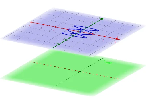
This GeoGebra example dynamically demonstrates the winding number of a plane curve around a given point, which counts how many times (with orientation) the curve loops around that point. The core mathematical concept is the winding number from complex analysis, defined as the path integral of the curve divided by 2πi, and intuitively visualized by counting intersections of the curve with a ray emanating from the point. The construction uses GeoGebra commands such as Sequence, Zip, CurveCartesian, Sphere, Intersect, Textfield, Vector, Point, and Locus to build parametric curves, discrete sampling, and interactive controls. It also employs 3D visualization aids (Sphere, Intersect) and input boxes for parameter adjustment. Suitable for university-level complex analysis, topology, or mathematical experimentation courses, as well as advanced high school enrichment to grasp the geometric meaning of curve orientation and looping.