
Syntractrice Curve Demonstration
Loading the math board and drawing, please wait…
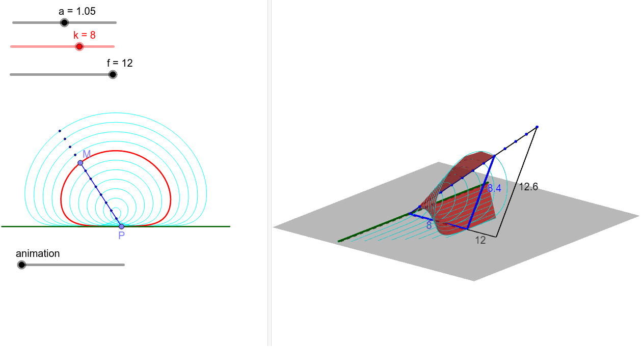
This example demonstrates the properties and construction process of the syntractrice curve, a complex mathematical figure. It involves core concepts like coordinate geometry, piecewise functions, symmetry, and transformations. The construction utilizes GeoGebra commands and objects such as CurveCartesian, Segment, Point, If, Surface, Sequence, and Dilate. Suitable for high school and above, it helps learners understand the intricacies of constructing and analyzing complex curves.
GeoGebra Commands & Parameters
CurveCartesian((a * (t - (k * tanh(t)))), (a * k / cosh(t)), t, (-f), f) → bSegment((-A), A) → pPoint(p) → PPoint(b, PathParameter[P]) → MpIf(d + 0.2 > f, f, d + 0.2) → maIf(d - 0.2 < (-f), (-f), d - 0.2) → miPoint(b) → MPoint(p, PathParameter[M]) → PmCurveCartesian((a * (t - (k * tanh(t)))), (a * k / cosh(t)), t, mi, ma) → ePoint(e) → MMSurface((a * (u - (v * tanh(u)))), v, (a * v / cosh(u)), u, (-f), fm, v, 0, k) → gSegment((x(P), 0, y(P)), (x(M), k, y(M))) → hSegment((x(P), k, y(P)), (x(M), k, y(M))) → jSegment(P, M) → cSequence(CurveCartesian[(a * (t - (i * tanh(t)))), (a * i / cosh(t)), t, (-f), f], i, 0, 12, 1) → liste2Segment((x(P), 0), (x(P), k)) → iSequence(CurveCartesian[(a * (t - (i * tanh(t)))), i, (a * i / cosh(t)), t, (-f), f], i, 0, k, 1) → liste3Segment((x(P), 0), (x(P), 12)) → lDilate(M_2, 12 / k, P_2) → M_3Segment((x(P), 12, 0), M_3) → mSequence(Dilate[M_3, i, P_2], i, 0, 1, 1 / 12) → liste4Segment(P_2, M_3) → nDilate(M, 12 / k, P) → M_1Sequence(Dilate[M_1, i, P], i, 0, 1, 1 / 12) → liste1