Surface Area Expressions: Visualizing Polyhedral Areas with Linear Programming

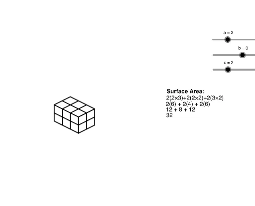
① This GeoGebra example dynamically illustrates how surface area expressions are formed from multiple planes enclosing a solid, linking algebraic formulas to geometric visualization. ② Core mathematical concepts include surface area computation, plane equations, linear programming (feasible regions and objective functions), dilation/affine transformations, and complex numbers for planar representation, along with sequence-generated lists. ③ Construction highlights: The Sequence command generates objects a, b, c and lists list1 through list6, likely storing plane equations or vertex coordinates; text objects text1–text5 display live area expressions, while sliders or inputs adjust parameters to update the figure and numeric values in real time. ④ Suitable for high school to early college students, this resource aids in understanding surface area derivation in solid geometry, the interplay between constraints and optimization in linear programming, and parametric modeling in dynamic mathematics software.