
Standard Deviation Measure of Spread
Loading the math board and drawing, please wait…
In collections
Continuous Random Variables
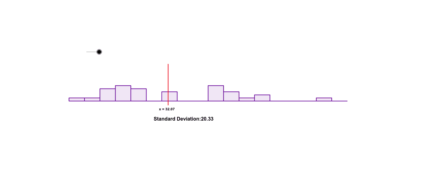
This example illustrates the standard deviation to show the dispersion of a dataset. Key concepts include standard deviation and mean. GeoGebra commands used include Sort, Element, SampleSD, Text, and Mean. Suitable for statistics education and presentations.
GeoGebra Commands & Parameters
Sort({9 * Random[1, a], 8 * Random[1, a], 5 * Random[1, a], 8 * Random[1, a], 5 * Random[1, a], 9 * Random[1, a], 8 * Random[1, a], 9 * Random[1, a], 5 * Random[1, a], 9 * Random[1, a], 8 * Random[1, a], 8 * Random[1, a], 5 * Random[1, a], 2 * Random[1, a], 5 * Random[1, a], 9 * Random[1, a], 5 * Random[1, a], 8 * Random[1, a], 6 * Random[1, a], 9 * Random[1, a], 8 * Random[1, a], 5 * Random[1, a], 9 * Random[1, a], 6 * Random[1, a], 4 * Random[1, a], 3 * Random[1, a], 2 * Random[1, a], 2 * Random[1, a], 2 * Random[1, a], 2 * Random[1, a]}) → list1Element(list1, 1) → bSampleSD(list1) → StandardElement(list1, 30) → dText("Standard Deviation:" * c) → text1Mean(list1) → hPoint(i) → APoint(i) → BSegment(A, B) → jText("x = " * h) → text2Histogram({0, 5, 10, 15, 20, 25, 30, 35, 40, 45, 50, 55, 60, 65, 70, 75, 80, 85, 90}, list1, false) → g