Slope Fields and Euler's Method: Interactive Visualization of Differential Equat

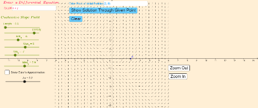
This GeoGebra example demonstrates how to visualize first-order differential equations using slope fields and approximate solutions via Euler's method. The core mathematical concepts include differential equations, slope fields, numerical integration, step size, and error analysis. The construction uses GeoGebra commands such as Textfield and SlopeField to create an interactive interface, with sliders or input boxes controlling the function f, slope field density, and the x/y ranges (Min_x, Max_x, Min_y, Max_y). Buttons (button1 to button9) trigger Euler iterations, generating points A, A1 to A5 and corresponding Δy increments, and finally plotting the Euler polygonal path. This tool is suitable for high school seniors or university students beginning differential equations, helping them understand the relationship between slope fields and numerical solutions, explore the effect of step size on accuracy, and serve as a classroom demonstration aid.