Scatter Plot and Linear Regression Analysis

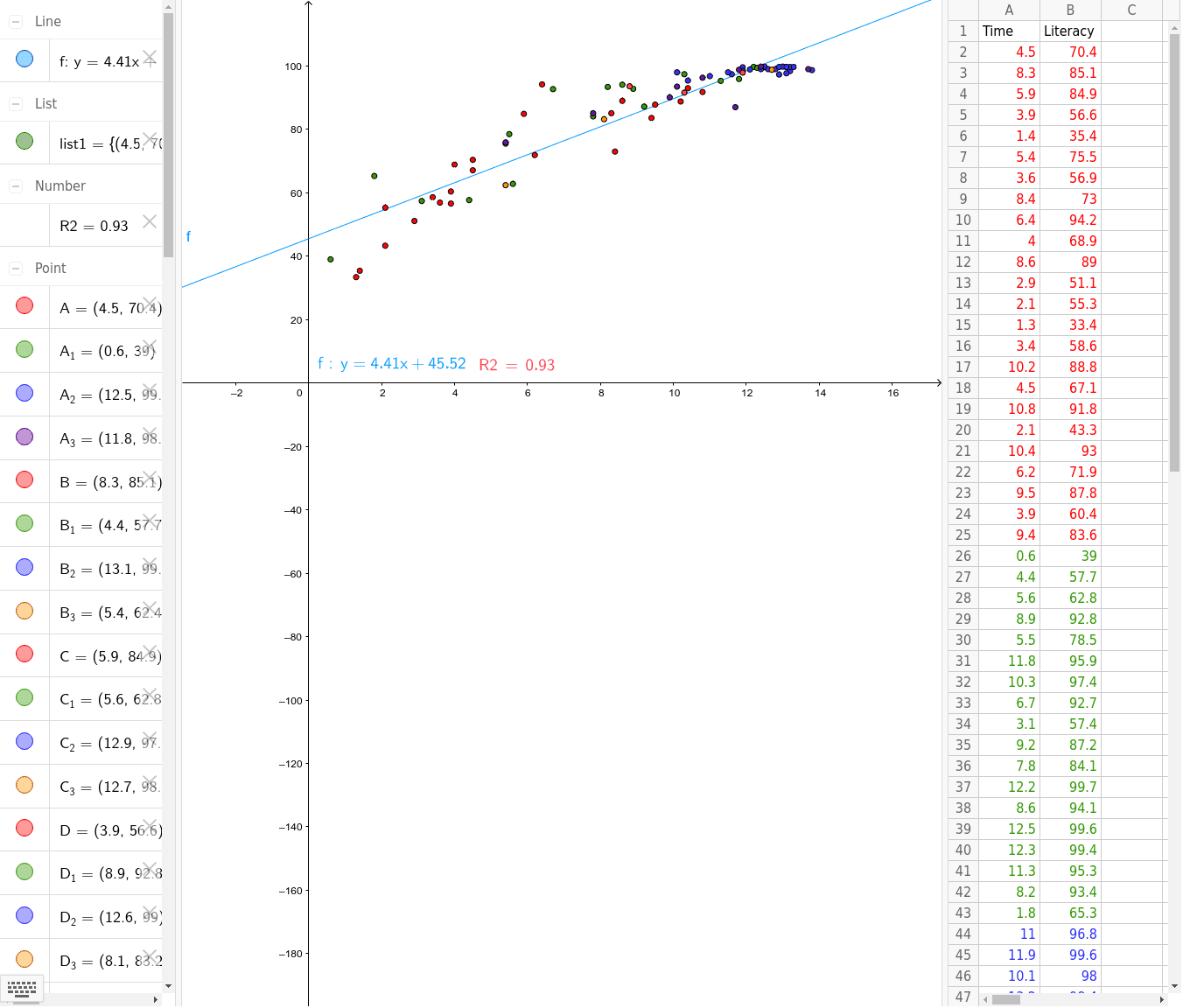
This GeoGebra example demonstrates the use of scatter plots for data distribution visualization and linear regression analysis, visually presenting correlation trends between variables. Core mathematical concepts involved include Pearson's product-moment correlation coefficient (PMCC), linear regression line fitting, matrix data structures, and quadratic function relations. Key construction elements include the use of the FitLineY command for best-fit line calculation, the PMCC command for quantitative correlation assessment, and the LaTeX command for formula rendering. The construction summary indicates the creation of a series of data point objects from A1 to A25 and B1 to B15, used to store and visualize multidimensional samples. This example is suitable for high school statistics, college data analysis, and coordinate geometry courses as an intuitive teaching tool.