
Quadratic Basketball Shot #4: Parabolic Trajectory Modeling
Loading the math board and drawing, please wait…
In collections
Parabolas
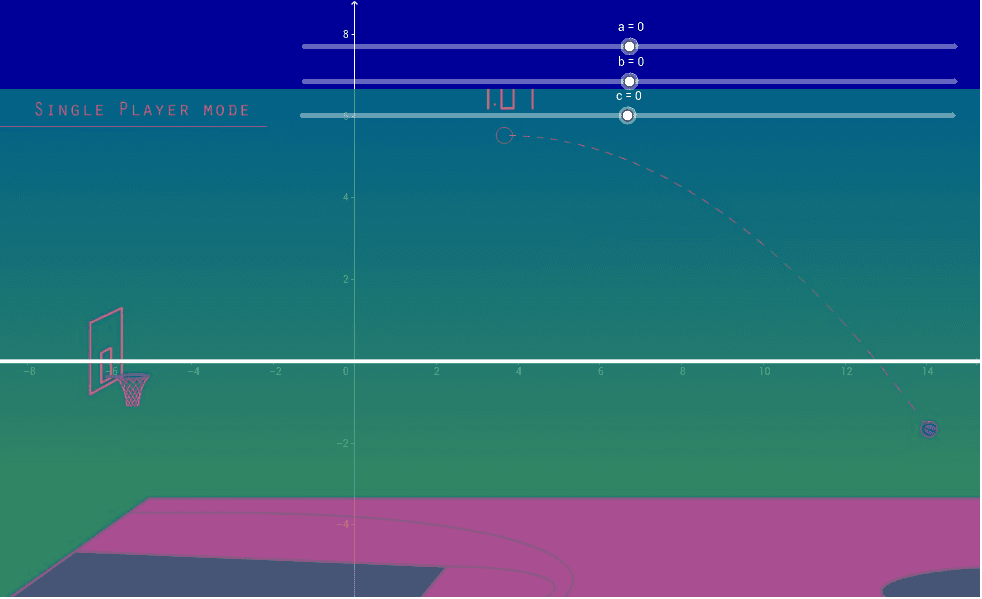
This GeoGebra example demonstrates how a quadratic function models the parabolic trajectory of a basketball shot, showing the ball's flight path under gravity and the conditions for scoring. Core mathematical concepts include quadratic functions, parabola graphs, projectile motion, the influence of function coefficients on graph shape, and quadratic function fitting. The construction uses objects a, b, c, d, e to define the quadratic equation, point A to mark the shooting position or hoop location, and pic1 as a background image of a basketball scene. Sliders enable dynamic adjustment of coefficients so the parabola aligns with the actual shot trajectory. It is suitable for high school mathematics teaching that integrates functions and geometry, classroom demonstrations, and student inquiry into quadratic function properties and real-world applications.
GeoGebra Commands & Parameters
Numeric a(0.0)Numeric b(0.0)Numeric c(0.0010)y = a * x^(2) + b * x + c(-b) / (2 * a)(e, a * e^(2) + b * e + c)
AI Drawing Prompt Reference
Create a coordinate-plane basketball shot diagram with a basketball-scene background image and a point marking the shooting position or hoop location. Draw a quadratic curve whose shape is controlled by three adjustable numeric parameters, representing the parabolic flight path of a basketball under gravity. Add another adjustable horizontal parameter that places a point on the curve, and show the x-coordinate of the curve's axis of symmetry. Emphasize that changing the parameters alters the opening direction, width, and position of the parabola so the curve can be aligned with the shot trajectory.
The prompt above was compiled from the original drawing commands and is for reference only.