
Proof of Perfect Square Trinomials
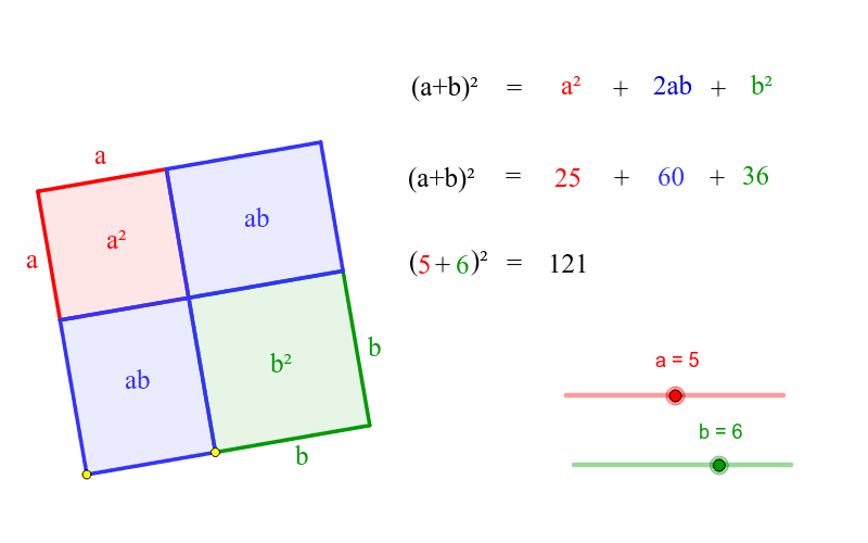
Loading the math board and drawing, please wait…
This example dynamically demonstrates the geometric interpretation and algebraic derivation of perfect square trinomials. It involves core concepts like quadratic functions, square roots, coordinate geometry, and geometric constructions. Key GeoGebra commands used include Circle, Point, Segment, Line, Intersect, OrthogonalLine, Polygon, and Midpoint, with objects like a, b, A, c, B to illustrate variable relationships. Suitable for high school mathematics education to enhance understanding of the connection between algebra and geometry and to develop students' ability to visualize abstract concepts.
GeoGebra Commands & Parameters
Circle(A, a) → cPoint(c) → BSegment(B, A) → dLine(A, B) → eCircle(B, b) → fIntersect(f, e) → C, DIntersect(c, e) → E, FOrthogonalLine(A, d) → gOrthogonalLine(B, d) → hOrthogonalLine(D, e) → iSegment(B, D) → jCircle(D, b) → kIntersect(k, i) → G, HOrthogonalLine(H, i) → lIntersect(l, h) → IIntersect(l, g) → JCircle(I, a) → pIntersect(p, h) → K, LOrthogonalLine(K, h) → mIntersect(m, g) → MIntersect(i, m) → NOrthogonalLine(L, h) → nIntersect(g, n) → OIntersect(i, n) → PIntersect(h, l) → QPolygon(I, B, D, H) → Vieleck1, i_1, b_1, d_1, h_1Polygon(O, J, I, L) → Vieleck2, o, j_1, i_2, l_1Segment(O, I) → qSegment(L, J) → rSegment(I, D) → sSegment(H, B) → tSegment(P, I) → a_1Segment(L, H) → c_1Segment(J, B) → e_1Segment(I, A) → f_1Polygon(L, I, H, P) → Vieleck3, l_2, i_3, h_2, p_1Polygon(J, A, B, I) → Vieleck4, j_2, a_2, b_2, i_4Intersect(q, r) → RIntersect(c_1, a_1) → SIntersect(s, t) → TIntersect(f_1, e_1) → UMidpoint(l_1) → VMidpoint(o) → WMidpoint(d_1) → ZMidpoint(j) → A_1