
Projectile Motion Simulation
Loading the math board and drawing, please wait…
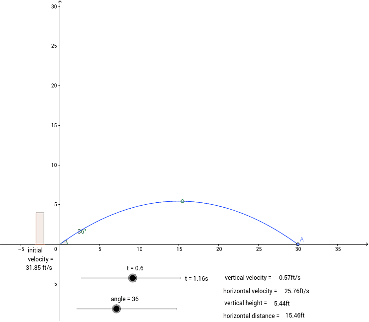
This example demonstrates the principles of projectile motion, allowing students to adjust initial velocity to achieve a target distance. It involves vector analysis, function graphing, and parametric equations. Constructed using GeoGebra commands like Point, Line, Function, and objects such as t, v_0, s_x, s_y, etc. Ideal for high school physics and mathematics education.
GeoGebra Commands & Parameters
Point({0, 0}) → wPoint({2, 0}) → vLine(w, v) → aPoint(a) → APoint({s_x, s_y}) → PFunction(tan(angle * π / 180) * x - 32.15 / (2 * v_0^(2) * cos(angle * π / 180)^(2)) * x^(2), 0, s_xend) → jPoint({2, 2 * tan(angle * π / 180)}) → uAngle(v, w, u) → αPoint({-3, 0}) → bPoint({-2, 0}) → cPoint({-3, v_0 / 8}) → dPoint({-2, v_0 / 8}) → fPolygon(c, f, d, b) → poly1, c_1, f_1, d_1, b_1
AI Drawing Prompt Reference
Draw a diagram of projectile motion, including a starting point and a target point, with a line connecting them. Show the trajectory of the projectile as a parabola starting from the initial point, passing through a point in the air, and landing at the target point. Add an angle to indicate the launch angle. Below, draw a rectangle representing one-eighth of the initial velocity.
The prompt above was compiled from the original drawing commands and is for reference only.