
Problem 20 (a): Price on Horizontal Axis - Demand and Supply Linear Functions
Loading the math board and drawing, please wait…
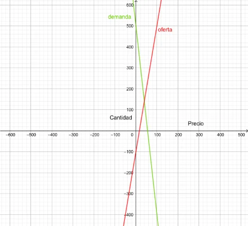
① This example demonstrates plotting demand and supply curves in a Cartesian coordinate system with price on the horizontal axis (independent variable), showing the geometric position of the market equilibrium point. ② Core mathematical concepts include linear functions, linear equations, linear regression ideas, and solving the intersection of two straight lines, applied to the classic economic model of demand and supply. ③ Construction highlights: from the construction summary, the GeoGebra objects 'demanda' (demand), 'oferta' (supply), and two text labels 'text1' and 'text2' are used; linear function expressions are entered to generate the lines, and text tools annotate curve names or key points. ④ Suitable for high school or early college courses bridging mathematics and economics, helping students understand linear function graphs, line intersections, and equilibrium price/quantity relationships, as well as serving as an intuitive introduction to linear regression applications.
GeoGebra Commands & Parameters
y = 500 - (9 * x)y = -100 + (6 * x)
AI Drawing Prompt Reference
Draw a demand curve and a supply curve. The demand curve follows the equation y = 500 - 9x, and the supply curve follows y = -100 + 6x. First, enter the equation for the demand curve, then enter the equation for the supply curve. After that, label the names of these curves and indicate the market equilibrium point on the graph.
The prompt above was compiled from the original drawing commands and is for reference only.