
Noticing Patterns: Interactive Exploration of Random Data and Statistical Fittin
Loading the math board and drawing, please wait…
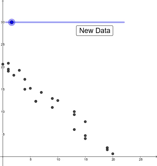
① This example demonstrates how to generate random scatter data and fit polynomial curves to reveal underlying patterns in statistics. ② Core mathematical concepts include correlation (PMCC), normal distribution, continuity, polynomial fitting (FitPoly), and three-dimensional vector representations. ③ Construction highlights: uses GeoGebra commands Random, If, PMCC, and FitPoly; objects include scatter plot, deviation, intercept, and numerous variables (A-Z) for dynamic parameter adjustment. ④ Suitable for high school to undergraduate courses in statistics and data analysis, this interactive tool helps students explore randomness, goodness-of-fit, and pattern recognition, bridging statistical inference with function approximation.
GeoGebra Commands & Parameters
Random(0, 20) → b_1If(scatter ≟ 0, 10.5, 1 / ((5 * scatter))) → deviationIf(scatter > 0, Random[0, 3], scatter < 0, Random[22, 25], scatter ≟ 0, Random[5, 15]) → interceptRandom(0, 20) → aRandom(0, 20) → a_1Random(0, 20) → wRandom(0, 20) → vRandom(0, 20) → uRandom(0, 20) → tRandom(0, 20) → sRandom(0, 20) → rRandom(0, 20) → qRandom(0, 20) → pRandom(0, 20) → oRandom(0, 20) → nRandom(0, 20) → mRandom(0, 20) → lRandom(0, 20) → kRandom(0, 20) → jRandom(0, 20) → iRandom(0, 20) → hRandom(0, 20) → gRandom(0, 20) → fRandom(0, 20) → eRandom(0, 20) → dRandom(0, 20) → cRandom(0, 20) → bPMCC(list) → correlationFitPoly(list, 1) → g_1
AI Drawing Prompt Reference
Create a set of random scatter points and fit a polynomial curve to reveal underlying patterns. First, generate some random numbers for the x and y coordinates of the scatter points, then calculate the deviation for each point, determine the intercept, and finally use PMCC to calculate the correlation coefficient and fit a polynomial curve.
The prompt above was compiled from the original drawing commands and is for reference only.