Normal Distribution & Cumulative Probability

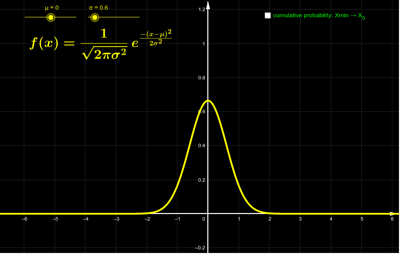
This example demonstrates the calculation and visualization of cumulative probability under a normal distribution curve. Key math concepts include Normal Distribution, Probability, Polygons, Upper and Lower Sum or Riemann Sum, Expected Value, Geometry, and Rational Numbers. The construction uses GeoGebra commands like Intersect, Point, Integral, and Segment, with objects such as μ, σ, f, A-F, a-c, I-J, T, text1-text2. It is suitable for high school and above students learning about probability statistics and integral applications in normal distributions.