
Normal Distribution and Tail Probabilities
Loading the math board and drawing, please wait…
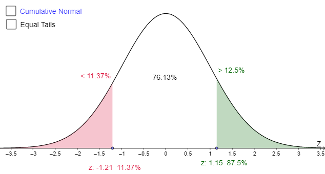
This example demonstrates the normal distribution curve and the calculation and visualization of tail probabilities. Key math concepts include normal distribution, probability density function, definite integral, and tail probability. GeoGebra commands and objects like Point, OrthogonalLine, Intersect, Midpoint, Textfield, Polygon, and Vector are used to construct the distribution curve, integral regions, intersection points, and text annotations. Suitable for high school and above students in mathematics and statistics to understand the properties of continuous random variables and probability calculations.
GeoGebra Commands & Parameters
Point(xAxis) → xrPoint(xAxis) → xlOrthogonalLine(xl, xAxis) → llOrthogonalLine(xr, xAxis) → lrIntersect(cn, ll, (-1.206857142857144, 0.1137435825015205)) → ClIntersect(nd, ll, (-1.206857142857144, 0.48275206426313805)) → NlIntersect(nd, lr, (1.15035, 0.5159979113655235)) → NrIntersect(cn, lr, (1.150349380376008, 0.875)) → CrMidpoint(Nl, Nr) → NmTextfield(alpha) → alphaBPolygon((-0.1, y(Zl)), (0.1, y(Zl)), (0.1, y(Zr)), (-0.1, y(Zr))) → mid, b, c, d, ePolygon((-0.1, 0), (0.1, 0), (0.1, 1), (-0.1, 1)) → m, m_2, m_3, m_4, m_5Vector(Zl, (-0.1, y(Zl))) → zlVector(xr, Zr) → zrVector(Zr, (0.1, y(Zr))) → mrVector(xl, Zl) → ml