Multivariate Limits Example 2: Visualizing Path-Dependent Approach

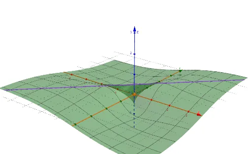
This GeoGebra example demonstrates the concept of limits for multivariate functions by visualizing a surface and multiple parametric curves approaching a target point. It highlights how the limit value can depend on the chosen path, a key subtlety in multivariable calculus. The construction uses the CurveCartesian command to define parametric curves, along with objects such as f, a, A, b, c, B, C, and d to control the surface, paths, and the point of approach. Users can manipulate sliders or dynamic points to see how different paths yield different limiting values, reinforcing the definition of a limit in higher dimensions. This resource is ideal for university-level calculus courses, serving as a visual aid for lectures or as an interactive tool for students to explore path-dependent limits and the non-uniqueness of limits when they do not exist.