
Multiple Models for Proper Fractions
Loading the math board and drawing, please wait…
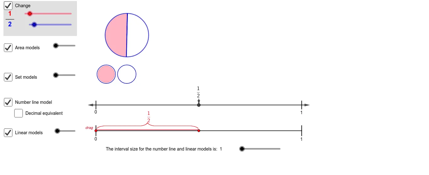
This example demonstrates various representations of proper fractions. It involves key mathematical concepts such as fractions and diagrams. Using GeoGebra commands like Segment, Point, Circle, and Polygon, it dynamically illustrates the geometric meaning of fractions. Suitable for middle school and above students to learn different representations of fractions.
GeoGebra Commands & Parameters
Segment(K_2, K_2 + (1 - num / denom, 0)) → linearModel1SegShiftPoint(linearModel1SegShift) → LinearModel1PtLCircle(R_1, T_1) → Circle_{model}Point(Circle[R_1, 0.105]) → C_2Polygon(LinearModel1PtL + (0, -0.03), LinearModel1PtL + (num / denom, -0.03), LinearModel1PtL + (num / denom, 0.03), LinearModel1PtL + (0, 0.03)) → int1, a, b, c, eVector(NL_c, NL_l) → uVector(NL_c, NL_r) → vVector(FP_t, FP) → wSegment((1, 0.13), (1, 0.17)) → i_2Segment((0, 0.13), (0, 0.17)) → j_2Segment(R_1, C_2) → m_2Rotate(C_2, angle, R_1) → D_2CircleSector(R_1, C_2, D_2) → r_3Segment(R_1, D_2) → l_2Rotate(C_2, (360 / denom)°, R_1) → B_2Sequence(Segment[Rotate[C_2, ((360 * i / denom))°, R_1], R_1], i, 0, denom) → Angle_{divseq}Segment(K_2, L_2) → a_2Vector((0, 0.25), (0.1, 0.25)) → image_{vector}Sequence(Translate[pic1, Vector[(i * image_{vector})]], i, 0, denom - 1) → Set_{opencat}Sequence(Translate[pic2, Vector[(i * image_{vector})]], i, 0, num - 1) → Set_{closedcat}Sequence(Translate[pic3, Vector[(i * image_{vector})]], i, 0, denom - 1) → Set_{openstar}Sequence(Translate[pic4, Vector[(i * image_{vector})]], i, 0, num - 1) → Set_{closedstar}Polygon(R_8, F_2, G_2, E_2) → rect_{red}, r_8, f_4, g_4, e_4Segment(R_8, I_2) → b_2Segment(E_2, H_2) → n_2Segment(E_2, M_2) → a_3Segment(J_2, R_8) → b_3Polygon((0.045, 0.588), (0.045 + num / ((3 * denom)), 0.588), (0.045 + num / ((3 * denom)), 0.385), (0.045, 0.385)) → areaModel3polyFill, j, k, l, mPolygon((-0.4493678126189438, 0.486), (-0.0923678126189438, 0.486), (-0.0923678126189438, 0.656), (-0.4493678126189438, 0.656)) → fracBackground, d, f, g, hSegment(LinearModel1PtL + (0, 0.005), LinearModel1PtR + (0, 0.005)) → linearModel1LineSequence(Segment[(i, 0.13), (i, 0.17)], i, 0, 1, 1 / intervalHashMarks) → numLineHashMarksSequence(Segment[(i, 0), (i, 0.05)], i, 0, 1, 1 / intervalHashMarks) → linearHashMarksSequence(Circle[(0.05 + i, 0.3), 0.045], i, 0, (denom - 1) / 10, 0.1) → setCircleOpenSequence(Circle[(0.05 + i, 0.3), 0.04], i, 0, (num - 1) / 10, 0.1) → setCircleShadingSequence(Segment[(0.045 + i / 11, 0.388), (0.045 + i / 11, 0.588)], i, 0, denom) → Area_{rectdiv}Sequence(Segment[(0.044 + i / ((3 * denom)), 0.387), (0.044 + i / ((3 * denom)), 0.588)], i, 0, denom) → Area_{rect2}FractionText(1 / intervalHashMarks) → intervalValue