
Modeling with Linear Equations
Loading the math board and drawing, please wait…
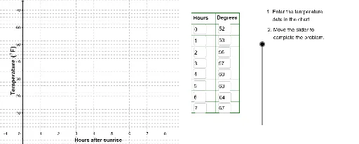
This example demonstrates the temperature changes recorded by a weather team every hour after sunrise in May. Using linear equations, students can understand the temperature changes over time. Key mathematical concepts include linear equations, coordinate geometry, and statistical characteristics. Dynamic temperature changes are shown using GeoGebra commands such as Corner, Polygon, and Textfield. Suitable for middle school and above students to learn about linear relationships in temperature changes.
GeoGebra Commands & Parameters
Corner(2) → Corn2Corner(3) → Corn3Polygon(Corn1, Corn2, Corn3, Corn4) → poly1, corn1, corn2, corn3, corn4Textfield(A2) → InA2Textfield(A3) → InA3Textfield(A4) → InA4Textfield(A5) → InA5Textfield(A6) → InA6Textfield(A7) → InA7Textfield(A8) → InA8Textfield(A9) → InA9Textfield(B9) → InB9Textfield(B8) → InB8Textfield(B7) → InB7Textfield(B6) → InB6Textfield(B5) → InB5Textfield(B4) → InB4Textfield(B3) → InB3Textfield(B2) → InB2Sequence(Segment[(9.5, 10 + (6.5 * j)), (12.2, 10 + (6.5 * j))], j, 0, 9) → LnListSequence(Segment[(9.5 + (1.35 * j), 10), (9.5 + (1.35 * j), 68.5)], j, 0, 2) → LnList2Line(I, J) → FitLineVerticalText("\text{Temperature (}°\text{F)}") → DownLegend
AI Drawing Prompt Reference
Draw a temperature change graph over time, with the x-axis representing hours and the y-axis representing temperature in Fahrenheit. Use line segments to show hourly temperature changes and fit a linear trend line to illustrate the temperature trend over time. Add a legend to indicate the temperature unit.
The prompt above was compiled from the original drawing commands and is for reference only.