
Lotka-Volterra Predator-Prey Model by Juan Carlos Ponce Campuzano
Loading the math board and drawing, please wait…
In collections
UQ-Applied Mathematical Analysis
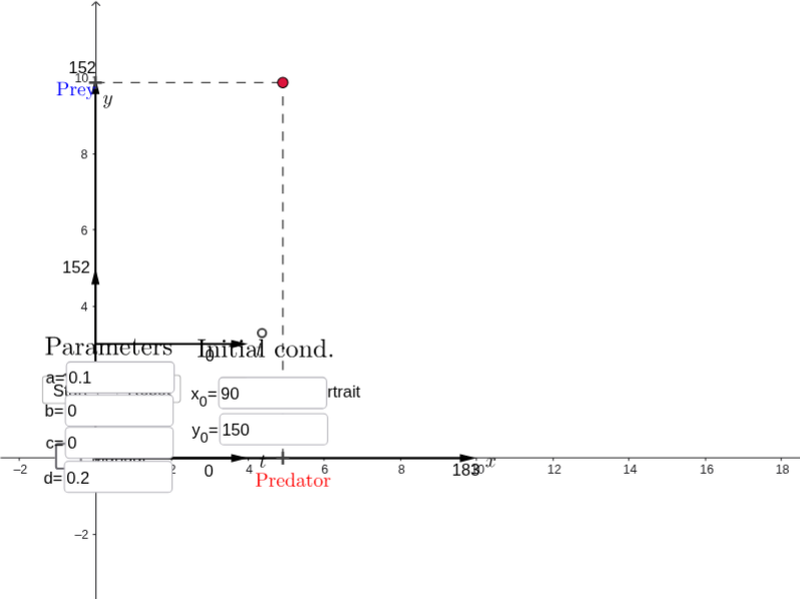
This example demonstrates the interaction between two species in a predator-prey relationship. Key mathematical concepts include differential equations and coordinate geometry. Using GeoGebra commands like SolveODE, Vector, and Intersect, the model dynamically shows the changes in predator and prey populations over time. Suitable for high school and above students studying population dynamics.
GeoGebra Commands & Parameters
SolveODE(G, F, x(B), y(B), t, step) → solutioneqLength(solutioneq) → npointsFirst(solutioneq, npoints) → list0Sequence(x(Element[list0, i]), i, 1, npoints) → list1Sequence(y(Element[list0, i]), i, 1, npoints) → list2Max(list1) → eMax(list2) → gSequence(((4 * i / N), (2 * Element[list1, i] / f)), i, 1, N) → list3Sequence(((4 * i / N), (2 * Element[list2, i] / h) + 3), i, 1, N) → list4Vector(C, E) → uVector(C, D) → vSequence(Sequence[Vector[((10 * j / f), (10 * k / h)), ((10 * (j + (scale * F(j, k))) / f), (10 * (k + (scale * G(j, k))) / h))], j, 0, xmax, xstep], k, 0, ymax, ystep) → list5Intersect(xAxis, yAxis) → IPoint(xAxis) → JPoint(yAxis) → KPoint(yAxis) → LPoint(yAxis) → MVector(I, J) → wVector(I, K) → iVector(L, M) → jVector(L, O) → kPolyLine(list3) → lPolyLine(list4) → mSequence(((10 * Element[list1, i] / f), (10 * Element[list2, i] / h)), i, 1, N) → list6Segment(T, B') → nSegment(S, B') → pSegment(R, P) → qSegment(P, Q) → rTextfield(a) → InputBox1Textfield(b) → InputBox2Textfield(c) → InputBox3Textfield(d) → InputBox4Textfield(A_0) → InputBox5Textfield(B_0) → InputBox6
AI Drawing Prompt Reference
Create a predator-prey model diagram in a coordinate plane with four parameter input boxes and two initial-population input boxes. Plot two time-series polylines derived from the differential-equation solution, one for prey and one for predator, scaled to the axes. Add a vector-field grid in the phase plane whose arrows are determined by the model equations, showing population change directions. Include points on the axes, several vectors anchored to those points, and line segments connecting related points to illustrate the dynamic relationship.
The prompt above was compiled from the original drawing commands and is for reference only.