
Logarithmic Function Transformation Exploration
Loading the math board and drawing, please wait…
In collections
Graph Transformations
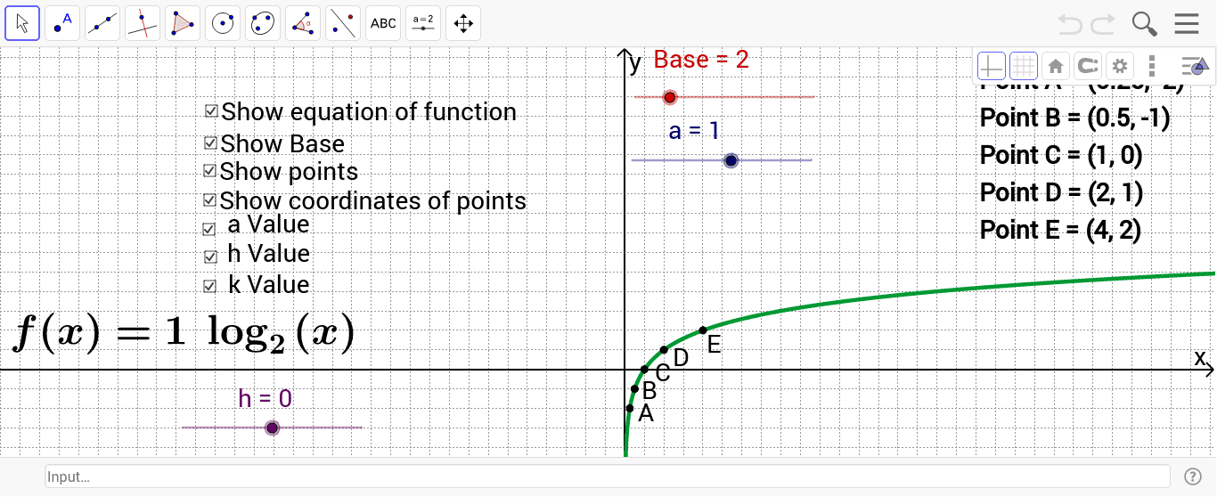
This example demonstrates how the graph of a logarithmic function changes with parameters k, h, and Base. It involves core math concepts like logarithmic function properties, graphical translation transformations, and parameter impact analysis. GeoGebra commands used include objects k, h, Base, a, f, A, B, D, E, a_1, b, C, Show, c, text1, d, e, g, h_1, text2, text3, text4, for dynamic graph display and parameter variation. Suitable for high school mathematics teaching to help students visually understand the rules of logarithmic function graph transformations.
GeoGebra Commands & Parameters
Numeric k(0.0)Numeric h(0.0)Numeric Base(2.0)Numeric a(1.0)f(x) = a * log(Base, x - h) + k(Base^(-2) + h, -2 * a + k)(Base^(-1) + h, -1 * a + k)(Base + h, a + k)(Base^(2) + h, 2 * a + k)Boolean a_1(true)Boolean b(true)(1 + h, k)Boolean c(true)Boolean d(true)Boolean e(true)Boolean g(true)Boolean h_1(true)
AI Drawing Prompt Reference
Draw a logarithmic function graph to show how parameters k, h, and Base affect the graph. Start with the basic logarithmic function, then apply vertical shifts with k, horizontal shifts with h, and observe changes by altering the Base. Mark key points on the graph such as x=Base^(-2), x=Base^(-1), x=1, x=Base, x=Base^2, and label their corresponding y-values to illustrate how parameter changes impact the graph's position and shape.
The prompt above was compiled from the original drawing commands and is for reference only.