Linear Regression with One Variable: Interactive Fitting Demonstration

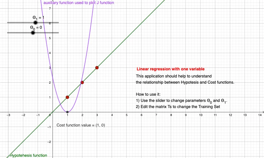
This GeoGebra example demonstrates interactive one-variable linear regression, showing how a regression line fits a set of data points and how the line adjusts as parameters change. Core mathematical concepts include the simple linear regression model y = Θ₀ + Θ₁x, the cost function J (mean squared error), parameter estimation for intercept and slope, and the geometric interpretation of least-squares fitting. The construction uses GeoGebra commands Length, Cell, Point, and PointList, together with objects such as Ts, m, Θ₁, Θ₀, h₀, a, J, b, c, j, E, L₁, L1, testo1, and testo2 to build points, segments, and dynamic text displays. It is suitable for high school statistics, introductory college data analysis, and machine learning preparatory courses, supporting classroom demonstration, inquiry-based learning, and visualization of regression principles.