
Linear Regression Visualizer - Residual Sum of Squares
Loading the math board and drawing, please wait…
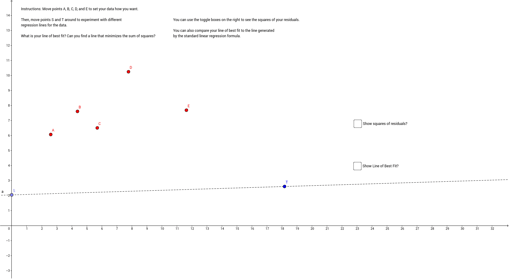
This example demonstrates the calculation and visualization of the residual sum of squares in linear regression. Key math concepts include linear regression, residual sum of squares, and least squares method. It constructs data points, regression lines, and residuals using GeoGebra commands like Point, Line, OrthogonalLine, Intersect, Polygon, FitLineY, RSquare. Suitable for high school and above students to understand evaluation metrics of linear regression models.
GeoGebra Commands & Parameters
Point(yAxis) → SLine(S, T) → aOrthogonalLine(B, xAxis) → bOrthogonalLine(C, xAxis) → cOrthogonalLine(A, xAxis) → dOrthogonalLine(D, xAxis) → eOrthogonalLine(E, xAxis) → fIntersect(a, b) → HIntersect(d, a) → IIntersect(c, a) → JIntersect(a, e) → KIntersect(a, f) → LPolygon(H, B, 4) → poly1, g, h, i, j, M, NPolygon(I, A, 4) → poly2, k, l, m, n, O, PPolygon(J, C, 4) → poly3, p, q, r, s, Q, RPolygon(K, D, 4) → poly4, t, a_1, b_1, c_1, S_1, T_1Polygon(L, E, 4) → poly5, d_1, e_1, f_1, g_1, U, V_1FitLineY(DataSet) → h_1Intersect(h_1, b) → FIntersect(h_1, c) → GIntersect(h_1, d) → ZIntersect(h_1, e) → A_1Intersect(h_1, f) → B_1Polygon(F, B, 4) → poly6, i_1, j_1, k_1, l_1, C_1, D_1Polygon(G, C, 4) → poly7, m_1, n_1, p_1, q_1, E_1, F_1Polygon(Z, A, 4) → poly8, r_1, s_1, t_1, a_2, G_1, H_1Polygon(A_1, D, 4) → poly9, b_2, c_2, d_2, e_2, I_1, J_1Polygon(B_1, E, 4) → poly10, f_2, g_2, h_2, i_2, K_1, L_1RSquare({(-3, 2), (-2, 1), (-1, 3), (0, 4), (1, 2), (2, 4), (3, 3), (4, 5), (6, 4)}, (0.5 * x) + 2.5) → w