
Linear Regression and Residuals
Loading the math board and drawing, please wait…
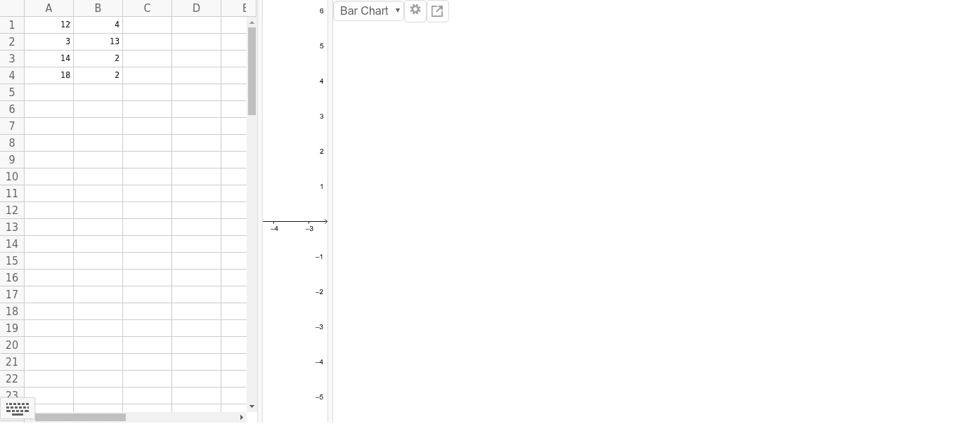
This example demonstrates the calculation and visualization of residuals in a linear regression model. Key math concepts include linear regression, residual analysis, and data fitting. It uses the GeoGebra command ResidualPlot with objects A1, B1, A2, B2, A3, B3, A4, B4 to construct the residual plot. Suitable for high school and above students learning about error analysis in linear regression.
GeoGebra Commands & Parameters
ResidualPlot({(12, 4), (3, 13), (14, 2), (18, 2)}, FitExp[{(12, 4), (3, 13), (14, 2), (18, 2)}]) →ResidualPlot({(12, 4), (3, 13), (14, 2), (18, 2)}, FitExp[{(12, 4), (3, 13), (14, 2), (18, 2)}]) →
AI Drawing Prompt Reference
Plot the points (12, 4), (3, 13), (14, 2), (18, 2), fit an exponential function through these points, and then draw the residual plot to analyze the fitting error.
The prompt above was compiled from the original drawing commands and is for reference only.