
Limits of Complex Functions
Loading the math board and drawing, please wait…
In collections
Mapping Diagrams to Visualize Complex Analysis
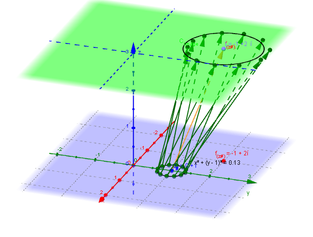
This example illustrates the concept of limits for complex functions. By adjusting parameters, observe the behavior of the function in the complex plane. Key mathematical concepts include complex numbers, limits, and functions. GeoGebra commands used include Sequence, CurveCartesian, Textfield, Vector, PointIn, Circle, etc. Suitable for high school mathematics education and learning.
GeoGebra Commands & Parameters
Sequence((δ * (cos(t) + (sin(t) * ί))) + x(z_0) + (y(z_0) * ί), t, -3.14159, 3.141592653589793, 0.5236) → z_*Sequence((x(Element[fz_*, k]), y(Element[fz_*, k]), height_{image}), k, 1, 12) → fpoint_*Sequence(Vector[Element[z_*, j], Element[fpoint_*, j]], j, 1, 12) → fvec_*CurveCartesian((δ * cos(t)), (δ * sin(t)), height_{image}, t, 0, 6.283185307179586) → dTextfield(fz_*) → inputBox1Vector(z_#, f_{(z#).}) → wTextfield(f_{(z#)}) → inputBox2CurveCartesian(t, 0, height_{image}, t, -5, 5) → XhCurveCartesian(0, t, height_{image}, t, -5, 5) → YhTextfield(z_*) → inputBox3PointIn(C_{image}) → LCircle(L, ε, Vector[(0, 0, 1)]) → f