Level Curves and Surfaces: Visualizing 3D Functions

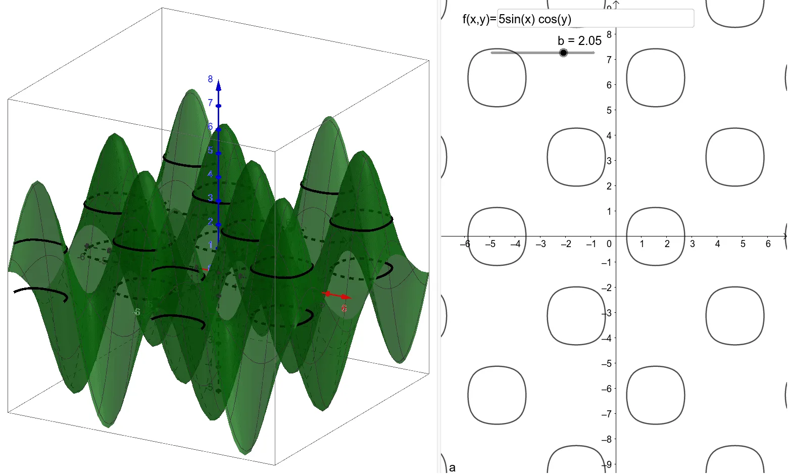
This GeoGebra example dynamically illustrates the relationship between level curves (contour lines) of a two-variable function and its corresponding 3D surface. It demonstrates how horizontal slices of a surface project onto the xy-plane as level sets, revealing the function's variation. Core mathematical concepts include level sets, contour lines, surfaces, and projections in multivariable calculus. The construction uses a Textfield for interactive input, a Plane object to create horizontal cutting planes, and the IntersectPath command to compute the intersection curves between the plane and the surface, generating the level curves. Key objects include the function f, parameters a and b, point A, and InputBox2, allowing dynamic adjustment of parameters to observe how the surface and its contours change together. This resource is suitable for high school to university-level mathematics education, particularly for introducing multivariable calculus and spatial analytic geometry, and serves well for classroom demonstrations or self-directed exploration of function shapes.