
Lazzarini's Pi Approximation
Loading the math board and drawing, please wait…
In collections
Pi Approximations
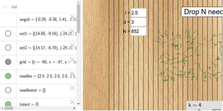
This example demonstrates Lazzarini's π approximation experiment by randomly throwing needles to estimate the value of π. It involves core mathematical concepts such as probability & statistics, geometric construction, limits, and integration. The construction utilizes GeoGebra commands and objects like Sequence, CountIf, Textfield, and Slider. Suitable for high school students and math enthusiasts studying probability statistics and calculus applications.
GeoGebra Commands & Parameters
Sequence(RandomUniform[-1.5707963267948966, 1.5707963267948966], i, 1, N) → angoliSequence((RandomUniform[(-10 * d), (10 * d)], RandomUniform[(-5 * d), (5 * d)]), i, 1, N) → ext1Sequence(Element[ext1, i] + ((l * sin(Element[angoli, i])), (l * cos(Element[angoli, i]))), i, 1, N) → ext2Sequence((x(Element[ext1, i]), x(Element[ext2, i])), i, 1, N) → xestrSequence(x = (i * d), i, -20, 20) → gridCountIf(floor(x(A) / d) ≠ floor(y(A) / d), A, xestr) → intersSequence(Segment[Element[ext1, i], Element[ext2, i]], i, 1, N) → needlesTextfield(d) → inputBox1Textfield(l) → inputBox2Textfield(NL) → inputBox3
AI Drawing Prompt Reference
This is a graphical representation of a pi approximation experiment based on probability and statistics. The graph includes a series of randomly thrown needles with fixed lengths, with needle tips distributed randomly around a circle. A circle is also shown, with its radius determined by a parameter d. Users can adjust the d value via a slider to observe changes in the probability of needle intersections. Intersecting needle points are marked, and statistical information is displayed. The construction order begins with generating random angles, calculating needle positions, drawing the circle and needles, and finally marking intersection points.
The prompt above was compiled from the original drawing commands and is for reference only.