Introduction to Systems of Linear Equations

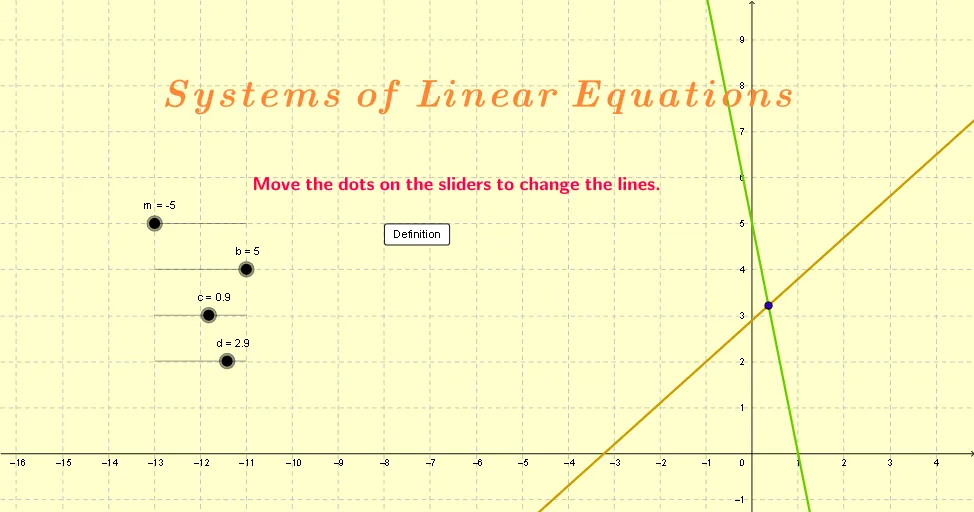
This example demonstrates how to understand and solve systems of linear equations through graphical methods. It involves core math concepts like linear equations, plane figures, variance, continuity, angles, and logarithmic functions. The construction uses GeoGebra commands like LaTeX for text, Intersect for finding intersections, and parameters such as m, b, a, c, d, e to build function graphs and intersection points. It is suitable for high school and above students to visually grasp the solution methods and geometric interpretations of linear systems.