
Introduction to Probability via Rolling a Die
Loading the math board and drawing, please wait…
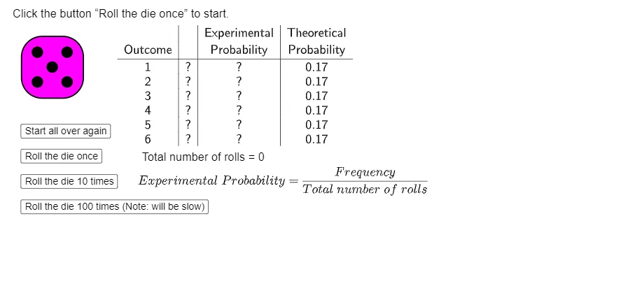
This example illustrates basic probability concepts by simulating the rolling of a die. It explores random variables, theoretical versus experimental probability, and discrete probability distributions. The GeoGebra construction uses commands such as Random, Frequency, Append, and TableText to create die graphics, control buttons for single rolls and resets, and dynamically display result tables and frequency counts. It is designed for high‑school or early university probability and statistics courses, as well as for mathematical modeling and experimental activities.
GeoGebra Commands & Parameters
Random(1, 6) → bFrequency(RollClass, RollResult) → RollFreqAppend("", Append["Frequency", RollFreq]) → ColFreqAppend("Experimental", Append["Probability", RollFreqFrac]) → ColFreqFracTableText({ColFaces, ColFreq, ColFreqFrac, ColTheoProb}, "|01110 _001000000 vc") → text2
AI Drawing Prompt Reference
Create an interactive chart simulating a die-rolling probability experiment. Show a six-sided die graphic in the center, with buttons for 'roll once' and 'reset'. Each roll updates the die face randomly and records frequencies, experimental probabilities, and theoretical probabilities (each 1/6) in a table below. The table has columns for face value, frequency, and probability, updating dynamically. The layout is clean, suitable for teaching, highlighting randomness and probability distribution comparison.
The prompt above was compiled from the original drawing commands and is for reference only.