
Introduction to Piecewise Functions
Loading the math board and drawing, please wait…
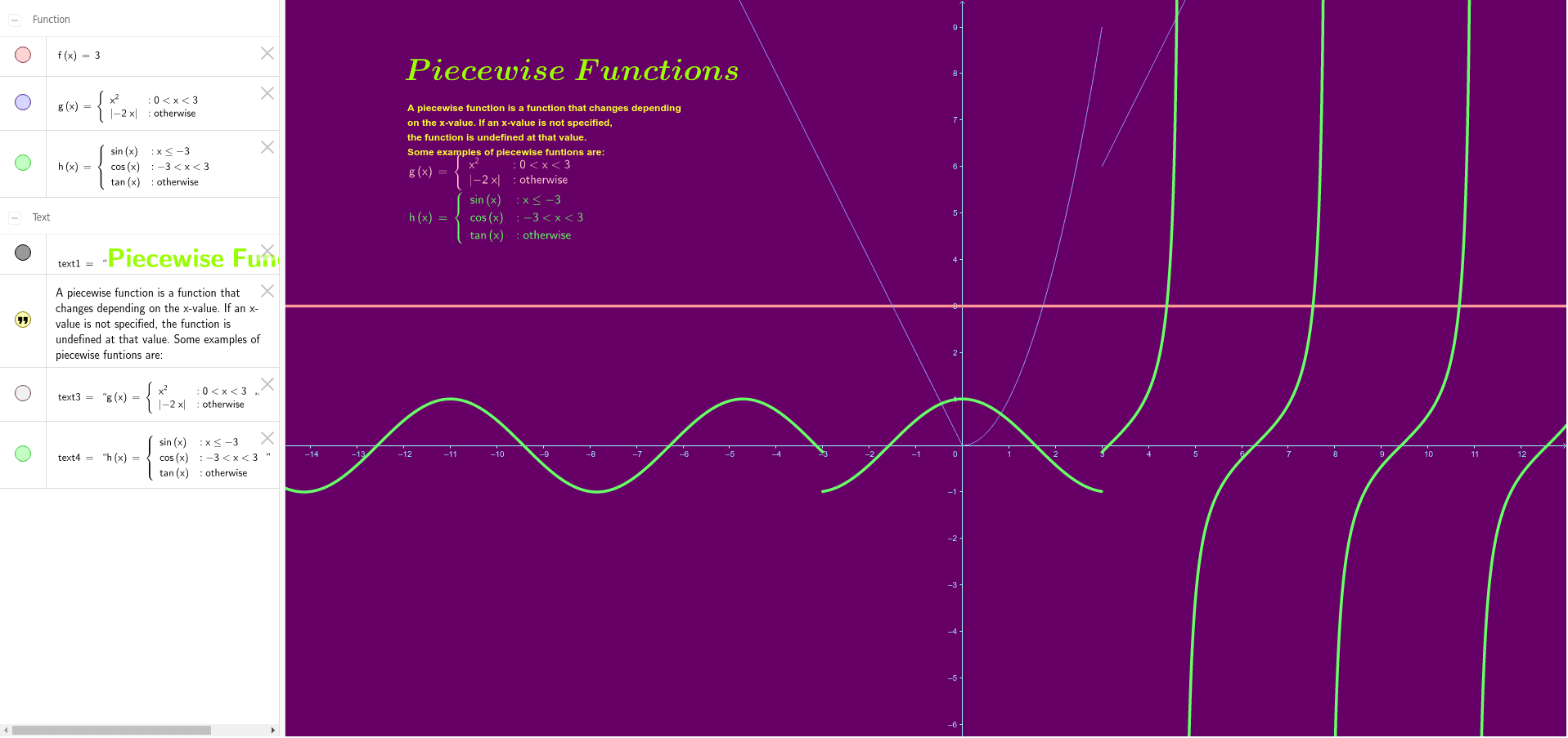
This example demonstrates how to graph piecewise functions and visualize their behavior across different intervals. Key math concepts include function definition, piecewise function properties, and analytical geometry graphing. Construction highlights involve using GeoGebra's If command for conditional logic, LaTeX for text formatting, and objects like text1, f, text2, g, text3, h, text4 for displaying functions and annotations. Suitable for high school mathematics education to help students understand the composition and graphical characteristics of piecewise functions.
GeoGebra Commands & Parameters
If(0 < x < 3, x^(2), abs(-2 * x)) → gLaTeX(g, true, true) → text3If(x ≤ -3, sin(x), If[-3 < x < 3, cos(x), tan(x)]) → hLaTeX(h, true, true) → text4
AI Drawing Prompt Reference
Draw a graph of two piecewise functions. The first function is defined as a parabola (x squared) for x between 0 and 3, and as the absolute value of negative 2x for all other x values. The second function has three pieces: sine for x less than or equal to -3, cosine for x between -3 and 3, and tangent for x greater than or equal to 3. Display both function formulas as mathematical text near their respective curves. Ensure the curves are clearly visible across intervals, with coordinate axes and grid lines shown.
The prompt above was compiled from the original drawing commands and is for reference only.