Interactive Visualization of Normal Distribution and Hypothesis Testing

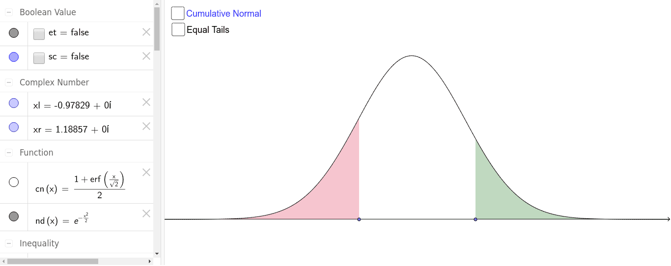
This GeoGebra example demonstrates the normal distribution curve in relation to hypothesis testing and boxplots, providing an interactive environment to explore distribution shapes and critical regions. Core mathematical concepts include the probability density function of the normal distribution, standard normal distribution, significance level α in hypothesis testing, critical Z-values, and left/right tail areas. Construction highlights: using GeoGebra commands such as Point, OrthogonalLine, Intersect, Midpoint, Polygon, Vector, Textfield, and Text to build auxiliary points, perpendicular lines, shaded regions, and dynamic labels. Multiple sliders (e.g., α, a, Z) allow users to adjust distribution parameters and test thresholds. This resource is suitable for high school and university statistics courses, helping students intuitively grasp properties of the normal distribution, rejection regions, and p-values, as well as the connection between boxplots and normal data.