Interactive Exploration of Polynomial Function End Behavior

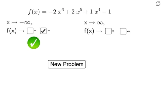
This GeoGebra example demonstrates the end behavior of polynomial functions—how the function values behave as x approaches positive or negative infinity. Key mathematical concepts include: relationship between polynomial degree and leading coefficient, odd/even function symmetry, and graphical interpretation of limits at infinity. Construction details: uses list objects to store polynomial coefficients, sliders (a, b, c, e) for parameter adjustment, buttons to trigger calculations, text displays for analysis results, and optional visual elements for辅助说明. Suitable for high school mathematics (functions and algebra) and pre-calculus students, ideal for classroom demonstration or student self-directed exploration of polynomial graphing characteristics.