
Integral as Accumulation of f(x) Values: Dynamic Visualization
Loading the math board and drawing, please wait…
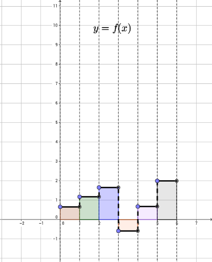
① This example dynamically visualizes the definite integral as the accumulation of function values f(x) over an interval, showing how areas sum to the integral. ② Core mathematical concepts include the geometric interpretation of definite integrals (area under a curve) and Riemann sums, involving functions, interval partitioning, and summation of rectangular areas. ③ Construction details: GeoGebra commands such as Point, OrthogonalLine, Intersect, Segment, Polygon, Vector, Translate, and Ray are used to create points, perpendicular lines, intersections, segments, polygons, and vectors, with translations and rays generating multiple rectangular strips; objects include A_0 to A_6, Y_0 to Y_5, etc., illustrating partitioning and accumulation. ④ Suitable for high school to college introductory calculus, helping students understand the relationship between integrals and area, and explore Riemann sum approximations.
GeoGebra Commands & Parameters
Point({0, 0}) → A_0Point({1, 0}) → A_1Point({2, 0}) → A_2Point({3, 0}) → A_3Point({4, 0}) → A_4Point({5, 0}) → A_5OrthogonalLine(A_0, xAxis) → uOrthogonalLine(A_1, xAxis) → gOrthogonalLine(A_2, xAxis) → hOrthogonalLine(A_3, xAxis) → iOrthogonalLine(A_4, xAxis) → jOrthogonalLine(A_5, xAxis) → kPoint(u) → Y_0Point(g) → Y_1Point(h) → Y_2Point(i) → Y_3Point(j) → Y_4Point(k) → Y_5OrthogonalLine(Y_0, u) → lOrthogonalLine(Y_1, g) → mOrthogonalLine(Y_2, h) → nOrthogonalLine(Y_3, i) → pOrthogonalLine(Y_4, j) → qOrthogonalLine(Y_5, k) → rIntersect(g, l) → AIntersect(h, m) → BIntersect(i, n) → CIntersect(j, p) → DIntersect(k, q) → EPoint({6, 0}) → A_6OrthogonalLine(A_6, xAxis) → sIntersect(r, s) → FSegment(Y_0, A) → tSegment(Y_1, B) → bSegment(Y_2, C) → dSegment(Y_3, D) → f_1Segment(Y_4, E) → i_1Segment(Y_5, F) → k_1Segment(A_6, A_5) → aSegment(A_4, A_3) → cSegment(A_2, A_1) → ePolygon(Y_0, A, A_1, A_0) → многоугольник1, y_0, a_1, a_2, a_0Polygon(Y_1, B, A_2, A_1) → многоугольник2, y_1, b_1, a_3, a_4Polygon(Y_2, C, A_3, A_2) → многоугольник3, y_2, c_1, a_5, a_6Polygon(Y_3, D, A_4, A_3) → многоугольник4, y_3, d_1, a_7, a_8Polygon(Y_4, E, A_5, A_4) → многоугольник5, y_4, e_1, a_9, a_{10}Polygon(Y_5, F, A_6, A_5) → многоугольник6, y_5, f_2, a_{11}, a_{12}Vector(A_0, Y_0) → vVector(A_1, Y_1) → wVector(A_2, Y_2) → u_1Vector(A_3, Y_3) → v_1Vector(A_4, Y_4) → w_1Vector(A_5, Y_5) → g_1Vector(A_0, A_1) → j_1Translate(A, j_1) → A'Translate(A', w) → A''Vector(A', A'') → l_1Translate(A'', j_1) → A'''Vector(A'', A''') → m_1Translate(A''', u_1) → GVector(A''', G) → n_1Translate(G, j_1) → G'Vector(G, G') → p_1Translate(G', v_1) → G''Vector(G', G'') → q_1Translate(G'', j_1) → G'''Vector(G'', G''') → r_1Translate(G''', w_1) → HVector(G''', H) → s_1Translate(H, j_1) → H'Vector(H, H') → t_1Translate(H', g_1) → H''Vector(H', H'') → u_2Translate(A_1, v) → IVector(A_1, I) → v_2Vector(I, A') → h_1Ray(I, A') → g_2Ray(A'', A''') → h_2Ray(G, G') → i_2Ray(G'', G''') → j_2Ray(H, H') → k_2Intersect(u, xAxis) → JSegment(J, I) → l_2Segment(I, A'') → m_2Segment(A'', G) → n_2Segment(G, G'') → p_2Segment(G'', H) → q_2Segment(H, H'') → r_2Segment(A, Y_1) → fSegment(B, Y_2) → s_2Segment(Y_3, C) → t_2Segment(D, Y_4) → b_2Segment(Y_5, E) → c_2