
Inputs and Outputs
Loading the math board and drawing, please wait…
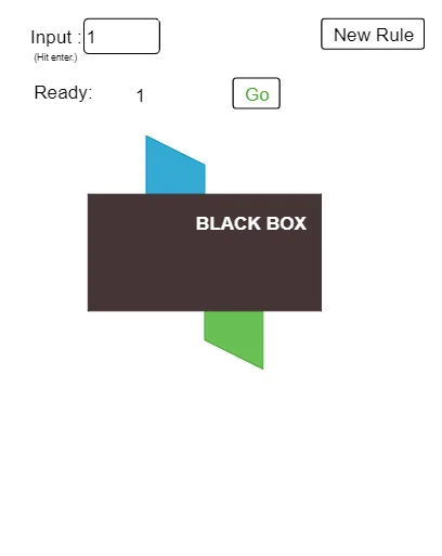
This example demonstrates the relationship between inputs and outputs, involving the concept of functions. Using GeoGebra commands such as Random, Textfield, and Polygon, a dynamic function graph is constructed. Suitable for middle school math education.
GeoGebra Commands & Parameters
Random(2, 5) → kRandom(2, 5) → aRandom(2, 5) → bRandom(2, 5) → hTextfield(inpt) → InputBox1Random(1, Length[list1]) → newRandom(0, 1) → fncPolygon(C, D, E, G) → poly1, c, d, e, g_1Translate(Polygon[C, C + (1, 0), C + (1, 0.5), C + (0, 1)], (1, 0)) → poly2Translate(Mirror[poly2, C + (2, 0)], Vector[C, D]) → poly3Element(inlist, 1) → A1Element(inlist, 2) → A2Element(inlist, 3) → A3Element(inlist, 4) → A4Element(inlist, 5) → A5Element(outlist, 1) → B1Element(outlist, 2) → B2Element(outlist, 3) → B3Element(outlist, 4) → B4Element(outlist, 5) → B5Element(inlist, 15) → A15Element(inlist, 14) → A14Element(inlist, 13) → A13Element(inlist, 12) → A12Element(inlist, 11) → A11Element(inlist, 10) → A10Element(inlist, 9) → A9Element(inlist, 7) → A7Element(outlist, 6) → B6Element(outlist, 7) → B7Element(outlist, 8) → B8Element(outlist, 9) → B9Element(outlist, 10) → B10Element(outlist, 11) → B11Element(outlist, 12) → B12Element(outlist, 13) → B13Element(outlist, 14) → B14Element(outlist, 15) → B15Element(inlist, 8) → A8Element(inlist, 6) → A6Random(1, Length[list2]) → ckn_0Sequence(F(i), i, -5, 5) → list3, {-2.5, -2, -1.5, -1, -0.5, 0, 0.5, 1, 1.5, 2, 2.5}Textfield(rule) → InputBox2Sequence(rule(i), i, -5, 5) → list4, {-5, -4, -3, -2, -1, 0, 1, 2, 3, 4, 5}Sequence(rule(Element[inlist, i]), i, 1, Length[inlist]) → list5, {}
AI Drawing Prompt Reference
Create a dynamic diagram illustrating the relationship between function inputs and outputs. Place an input box on the left and an output box on the right, connected by a function curve in the coordinate plane. The input box contains a list of numbers, and the output box shows the corresponding function results. Use polygons to represent the mapping process, with each input value linked to its output point via arrows or lines. The function curve is generated with random parameters, and the overall layout is clear for educational demonstration.
The prompt above was compiled from the original drawing commands and is for reference only.