Graphing Inequalities with Dynamic Visualization

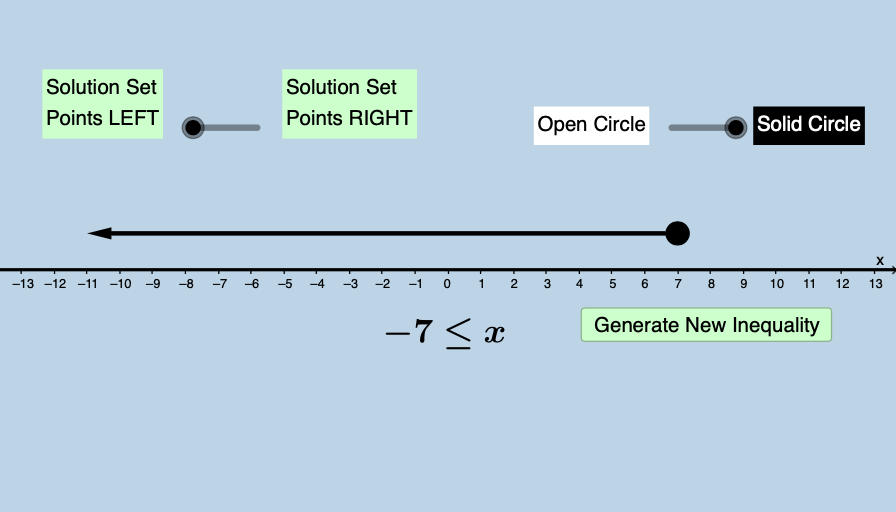
This GeoGebra example demonstrates the graphical representation of inequalities, showing how solution sets appear as shaded regions on the coordinate plane. The core mathematical concepts include linear inequalities, region partitioning, boundary lines, and the geometric meaning of solution sets. The construction uses the Random command to generate random points, DynamicCoordinates to update point positions interactively, and Vector objects to indicate directions or regions. Multiple text objects (text1 through text9) and a button (button1) provide labels and interactive controls, resulting in a complete graph with inequality regions, boundaries, and annotations. This resource is suitable for middle and high school students learning about inequality graphing, and can be used by teachers for classroom demonstrations or by students for self-exploration to connect algebraic expressions with their geometric interpretations.