Graphing in Polar Coordinates: Dynamic Parameters and Tangents

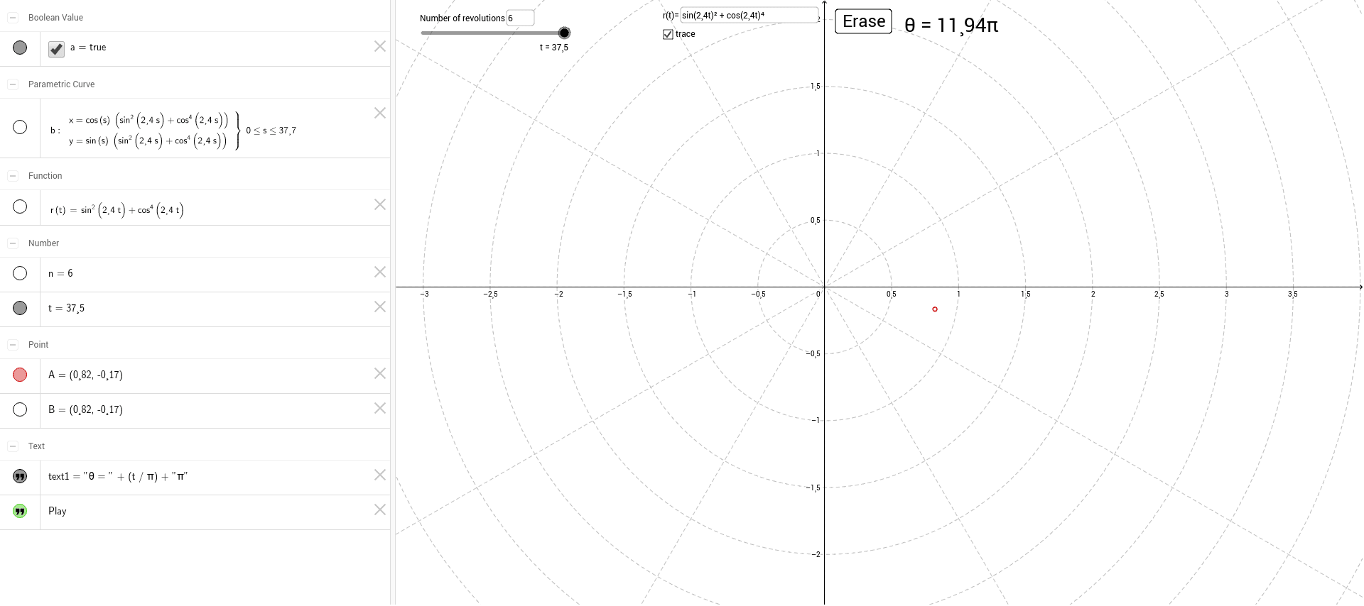
This example demonstrates plotting parametric curves in polar coordinates, with interactive controls to adjust parameters and observe changes in the graph. Core mathematical concepts include polar-to-Cartesian conversion, parametric curves, tangent lines, and vector multiplication. The construction uses GeoGebra's Textfield and button controls, along with the CurveCartesian command to generate curves, while dynamically displaying points, tangents, and incircles. Suitable for high school or early college students to understand polar graphing and parameter effects, and useful for classroom demonstrations.