
Geometric Visualization of Complex Roots of a Quadratic
Loading the math board and drawing, please wait…
In collections
Imagining Complex Roots
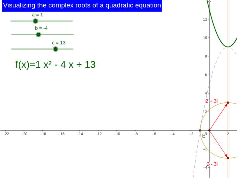
① This example shows how to visualize the two conjugate complex roots of a quadratic equation by geometric construction in the Cartesian plane. ② Core concepts: quadratic function graph, discriminant, complex‑plane representation, and conjugate symmetry. ③ Construction highlights: Intersect finds real‑axis intersections; OrthogonalLine, Mirror, and Circle build the symmetric circle; ComplexRoot directly yields the complex roots z₁, z₂; Vector displays modulus and argument. Key objects: coefficients a, b, c; function f; points A, B, Vx, P, d, C, f₁, E, F, e, G, H; discriminant; roots z_1, z_2; vectors u, v. ④ Suitable for high‑school elective complex‑number units, college algebra/geometry courses, classroom demos, and self‑study.
GeoGebra Commands & Parameters
Intersect(f, xAxis) → A, BOrthogonalLine(P, xAxis) → dIntersect(f, d) → CMirror(f, C) → f_1Intersect(f_1, xAxis) → E, FCircle(P, F) → eIntersect(xAxis, yAxis) → GIntersect(e, d, 2) → HComplexRoot(f) → z_1, z_2Vector(G, z_1) → uVector(G, z_2) → v
AI Drawing Prompt Reference
Draw a quadratic function graph and find the two intersection points A and B on the x-axis. Construct a vertical line d through point P, which intersects the function at point C. Mirror the function to get f₁, then find the two intersection points E and F of f₁ with the x-axis. Draw a circle e with center P and radius F, intersecting line d at point H. Use the quadratic function to directly obtain the two conjugate complex roots z₁ and z₂, and draw vectors u and v from point G to represent z₁ and z₂.
The prompt above was compiled from the original drawing commands and is for reference only.